MoE tutorial

Introduction

Motivation

现有大部分大语言模型均是基于 Transformer (Vaswani et al., 2017) 架构，scaling law (Hoffmann et al., 2022; Kaplan et al., 2020) 通过实验说明，大语言模型的表现与算力，数据，模型参数量息息相关。但是，对于 dense 模型来说，我们提高模型参数量时，必须同时提高所使用的算力。这就限制了大模型的 scaling law.

而 MoE 模型的解决方法为在计算时只激活部分参数，这样，我们就可以在同等激活参数量/算力下训练更大参数量的模型，从而达到更好地表现。因此，MoE 模型的核心思想在于

在使用相同的激活参数量/算力的情况下，提高模型总参数量，从而达到更好的表现。

Why MoE

选择 MoE 的原因有三点：效率, scaling law 以及表现。

Efficiency

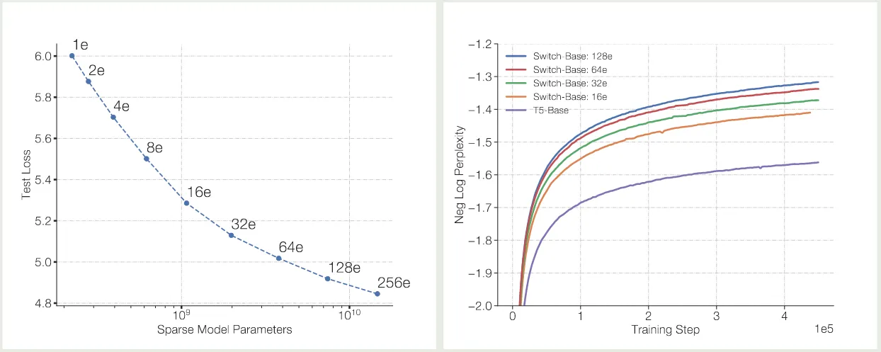
MoE 训练更加高效，如下图所示

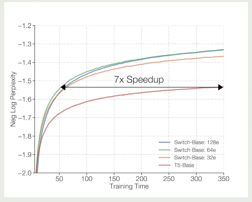
Comparison between MoE and dense models (Switch Transformer)

Switch Transformer (Fedus et al., 2022) 的实验结果说明，MoE model 的训练效率比 dense model 快 7 倍左右。其他模型也有类似结论。总的来说，MoE 模型相比于 dense 模型，训练效率更高。

(Zhao et al., 2025) 的计算开销如下所示 (4096 context length)

Model	Type	Size	Training Cost
DeepSeek-V2	MoE	236B	155 GFLOPS/Token
DeepSeek-V3	MoE	671B	250 GFLOPS/Token
Qwen-72B	Dense	72B	394 GFLOPS/Token
LLaMa-405B	Dense	405B	2448 GFLOPS/Token

更适合端侧部署TODO

Scaling Law

MoE 模型可以突破传统 scaling law 的限制，在算力固定的情况下，我们可以通过提高 MoE 模型的稀疏度来进一步提高模型的表现 (Tian et al., 2025)

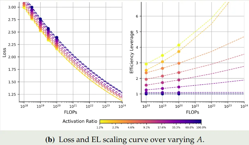
Impact of the activation ratio on loss and efficiency

如上图所示，在 FLOPs 给定的情况下，随着模型稀疏度的提高，模型的表现和效率都有提升

Performance

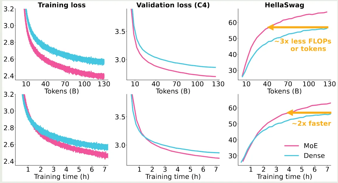
MoE 模型的表现更强，如下图所示，MoE 模型的训练，验证损失以及在下游任务上的表现均超过了 dense 模型

Timeline

下图展示了 MoE 模型的激活比例随时间的变化趋势，可以通过 “Parameters” 和 “Experts” 按钮独立控制显示两种激活比例（可同时显示）。圆圈大小代表模型总参数量。

MoE Activation Ratio Timeline

圆圈大小代表模型总参数量，悬停查看详情

可以看到，当前大部分模型的参数激活比例都在 $5\%$ 左右。从专家激活比例来看，DeepSeek-MoE 和 Hunyuan-A13B 的专家激活比例较高，而 Kimi-K2 和 LongCat 则使用了极低的专家激活比例。Kimi-K2 (Team et al., 2026) 认为提高专家个数可以提高模型表现，而 LongCat 则是使用了 phantom expert 机制。

Fedus, W., Zoph, B., & Shazeer, N. (2022). Switch transformers: scaling to trillion parameter models with simple and efficient sparsity. J. Mach. Learn. Res., 23(1).
Hoffmann, J., Borgeaud, S., Mensch, A., Buchatskaya, E., Cai, T., Rutherford, E., de Las Casas, D., Hendricks, L. A., Welbl, J., Clark, A., Hennigan, T., Noland, E., Millican, K., van den Driessche, G., Damoc, B., Guy, A., Osindero, S., Simonyan, K., Elsen, E., … Sifre, L. (2022). Training Compute-Optimal Large Language Models. https://arxiv.org/abs/2203.15556
Kaplan, J., McCandlish, S., Henighan, T., Brown, T. B., Chess, B., Child, R., Gray, S., Radford, A., Wu, J., & Amodei, D. (2020). Scaling Laws for Neural Language Models. https://arxiv.org/abs/2001.08361
Team, K., Bai, Y., Bao, Y., Charles, Y., Chen, C., Chen, G., Chen, H., Chen, H., Chen, J., Chen, N., Chen, R., Chen, Y., Chen, Y., Chen, Y., Chen, Z., Cui, J., Ding, H., Dong, M., Du, A., … Zu, X. (2026). Kimi K2: Open Agentic Intelligence. https://arxiv.org/abs/2507.20534
Tian, C., Chen, K., Liu, J., Liu, Z., Zhang, Z., & Zhou, J. (2025). Towards Greater Leverage: Scaling Laws for Efficient Mixture-of-Experts Language Models. https://arxiv.org/abs/2507.17702
Vaswani, A., Shazeer, N., Parmar, N., Uszkoreit, J., Jones, L., Gomez, A. N., Kaiser, L., & Polosukhin, I. (2017). Attention Is All You Need. Advances in Neural Information Processing Systems.
Zhao, C., Deng, C., Ruan, C., Dai, D., Gao, H., Li, J., Zhang, L., Huang, P., Zhou, S., Ma, S., Liang, W., He, Y., Wang, Y., Liu, Y., & Wei, Y. X. (2025, June). Insights into DeepSeek-V3: scaling challenges and reflections on hardware for AI architectures. Proceedings of the 52nd Annual International Symposium on Computer Architecture. 10.1145/3695053.3731412

Basic MoE

Definition

MoE 模型和 dense 模型的示意图如下，图源 OLMoE (Muennighoff et al., 2025)

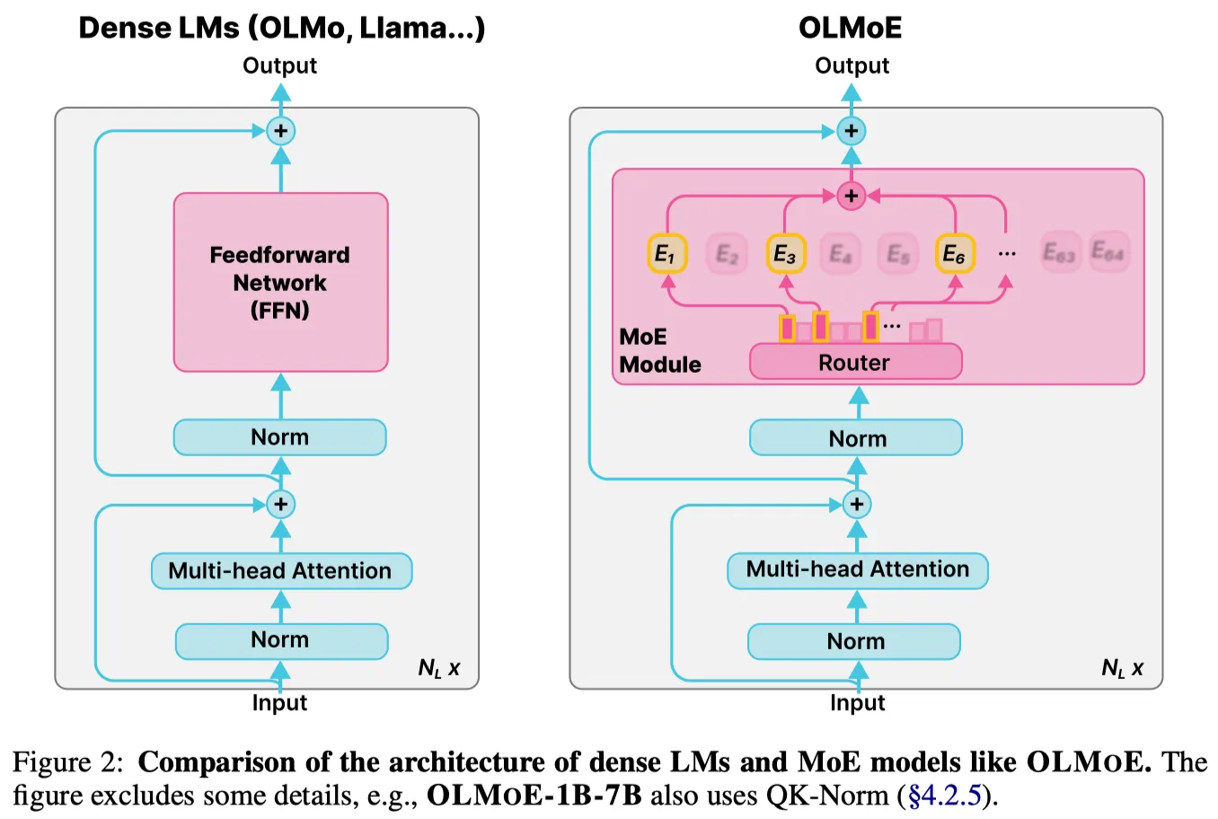
一个 MoE layer 包括两个模块：

Router：Router 负责为 token 指定合适的专家
Expert：Expert 负责处理 token

对于输入 $x\in\mathbb{R}^d$ , 我们假设有 $N$ 个 Expert，router 一般是一个 linear layer 再加上一个 gating function (softmax 或者 sigmoid，我们本文中使用 softmax), 其构建了 $\mathbb{R}^d\to\mathbb{R}^N$ 的映射，定义为：

G(x) =[G_1(x),\dots,G_N(x)] = \mathrm{softmax}(W_gx + b)\in\mathbb{R}^N

其中 $W_g\in\mathbb{R}^{N\times d}$ , $b\in\mathbb{R}^N$ 是可学习的参数， $G_{i}(x)$ 代表了当前 token $x$ 选择第 $i$ 个 Expert 的概率。

一般来说，Expert 会使用和 dense 模型一样的 MLP, 我们记为

E_i(x) = \mathrm{FFN}(x), \quad i = 1,\dots,N

接下来，基于 $G(x)$ 和 $E(x)$ , 我们会使用合适的方法来挑选 $K<N$ 个 Expert 出来，其中 $K$ 是给定的超参数，我们记挑选出来的 $K$ 个 Expert 的 index 为 $e_1,\dots,e_K$ , 即

e_i \in \{i\mid G_i(x)\in \mathrm{TopK}(G_i(x), K)\},\ i=1,\dots,K

这里 $\mathrm{TopK}$ 指的是概率值最高的 $K$ 个值。最终 MoE layer 的输出为

y = \sum_{i=1}^K\mathrm{Normalize}(G_{e_i}(x)) E_{e_i}(x)

这里 $\mathrm{Normalize}(\cdot)$ 代表我们对于输出进行归一化，即

\mathrm{Normalize}(G_{e_i}) = \frac{\exp(G_{e_i})}{\sum_{i=1}^K \exp(G_{e_i})},\quad i=1,\dots,K

Code

OLMoE implementation

class OlmoeSparseMoeBlock(nn.Module):
    def __init__(self, config):
        super().__init__()
        self.num_experts = config.num_experts
        self.top_k = config.num_experts_per_tok
        self.norm_topk_prob = config.norm_topk_prob
        self.gate = nn.Linear(config.hidden_size, self.num_experts, bias=False)
        self.experts = nn.ModuleList([OlmoeMLP(config) for _ in range(self.num_experts)])

    def forward(self, hidden_states: torch.Tensor) -> torch.Tensor:
        batch_size, sequence_length, hidden_dim = hidden_states.shape
        # hidden_states: (batch * sequence_length, hidden_dim)
        hidden_states = hidden_states.view(-1, hidden_dim)
        # router_logits: (batch * sequence_length, n_experts)
        router_logits = self.gate(hidden_states)

        routing_weights = F.softmax(router_logits, dim=1, dtype=torch.float)
        # routing_weights: (batch * sequence_length, top_k)
        # selected_experts: indices of top_k experts
        routing_weights, selected_experts = torch.topk(routing_weights, self.top_k, dim=-1)
        if self.norm_topk_prob:
            routing_weights /= routing_weights.sum(dim=-1, keepdim=True)
        # we cast back to the input dtype
        routing_weights = routing_weights.to(hidden_states.dtype)

        final_hidden_states = torch.zeros(
            (batch_size * sequence_length, hidden_dim), dtype=hidden_states.dtype, device=hidden_states.device
        )

        # One hot encode the selected experts to create an expert mask
        # this will be used to easily index which expert is going to be selected
        expert_mask = torch.nn.functional.one_hot(selected_experts, num_classes=self.num_experts).permute(2, 1, 0)

        # Loop over all available experts in the model and perform the computation on each expert
        for expert_idx in range(self.num_experts):
            expert_layer = self.experts[expert_idx]
            idx, top_x = torch.where(expert_mask[expert_idx])

            # Index the correct hidden states and compute the expert hidden state for
            # the current expert. We need to make sure to multiply the output hidden
            # states by `routing_weights` on the corresponding tokens (top-1 and top-2)
            current_state = hidden_states[None, top_x].reshape(-1, hidden_dim)
            current_hidden_states = expert_layer(current_state) * routing_weights[top_x, idx, None]

            # However `index_add_` only support torch tensors for indexing so we'll use
            # the `top_x` tensor here.
            final_hidden_states.index_add_(0, top_x, current_hidden_states.to(hidden_states.dtype))
        final_hidden_states = final_hidden_states.reshape(batch_size, sequence_length, hidden_dim)
        return final_hidden_states, router_logits

Muennighoff, N., Soldaini, L., Groeneveld, D., Lo, K., Morrison, J., Min, S., Shi, W., Walsh, E. P., Tafjord, O., Lambert, N., Gu, Y., Arora, S., Bhagia, A., Schwenk, D., Wadden, D., Wettig, A., Hui, B., Dettmers, T., Kiela, D., … Hajishirzi, H. (2025). OLMoE: Open Mixture-of-Experts Language Models. The Thirteenth International Conference on Learning Representations. https://openreview.net/forum?id=xXTkbTBmqq

MoE Design

Experts Design

Number of Experts

一般来说，专家个数越多，模型越稀疏，模型表现越好。扩展专家个数有两个方式：

直接增加专家个数，这会导致模型参数量上升，如 Switch Transformer (Fedus et al., 2022)
对已有的专家进行切分，将大专家切分为小专家，如 DeepSeekMoE (Dai et al., 2024)

Switch Transformer (Fedus et al., 2022) 也通过实验发现，增加专家个数可以显著提高模型的训练效率和表现，结果如下图所示

可以看到，当我们增加专家个数的时候，模型的表现是持续提升的。并且当我们增加专家个数之后，模型的训练效率也有所提升。

DeepSeekMoE (Dai et al., 2024) 提出了 fine-granularity expert 的概念，其做法是通过减少 expert 的大小在相同参数量的场景下使用更多的专家。实验结果如下图所示

DeepSeekMoE shared experts ablation study

可以看到，在稀疏度 (激活专家个数占总专家个数比例) 不变的情况下，提高专家的粒度，可以提高模型的表现。

OLMoE (Muennighoff et al., 2025) 对 DeepSeekMoE (Dai et al., 2024) 的这个观点进行了验证，结果如下图所示，

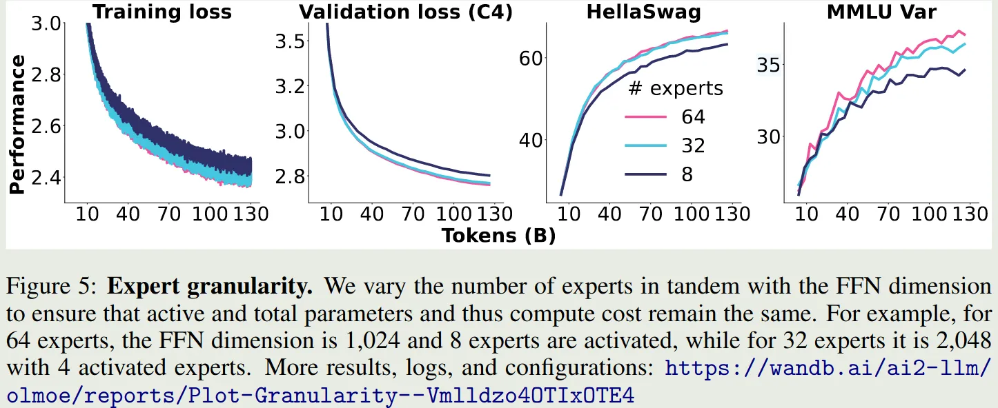
结果显示，当专家粒度从 8E-1A 扩展到 32E-4A 时，模型在 HellaSwag 上的表现提升了 $10\%$ , 但是进一步扩展到 64E-8A 时，模型的表现提升不到 $2\%$ , 这说明了无限制提升专家粒度对模型的提升越来越有限。

Kimi K2(Team et al., 2026) 探究了针对 MoE 模型 sparsity 的 scaling law, 结果也说明，提升 sparsity 可以提高模型的表现。因此，其相对于 DeepSeek-V3 (DeepSeek-AI et al., 2025) 使用了 $50\%$ 额外的的专家数。 Ling-mini-beta (Tian et al., 2025) 进一步验证了这个观点。

MiniMax-M2 (MiniMax et al., 2026) 也验证了细粒度专家可以提高模型表现的结论。

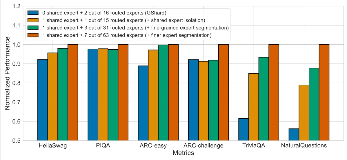
Shared Experts

Shared Expert 由 DeepSeekMoE (Dai et al., 2024) 提出，其基本思想为，固定某几个专家，响应所有的 token，这样可以让某些专家学习到共有的知识，而让其他的专家学习到特定的知识。这个方法随后被 Qwen1.5 (Q. Team, 2024), Qwen2 (Yang et al., 2024) , Qwen2.5 (Qwen et al., 2025) 以及 DeepSeek-V3 (DeepSeek-AI et al., 2025) 所采用。

DeepSeekMoE (Dai et al., 2024) 给出的实验结果如下

作者发现，当使用 shared experts 之后，模型在大部分 benchmark 上的表现都有所提升。

OLMoE (Muennighoff et al., 2025) 在 32 个专家下进行了实验，比较了 4 个激活专家和 3 个激活专家 +1 个共享专家两种设置的表现，结果如下：

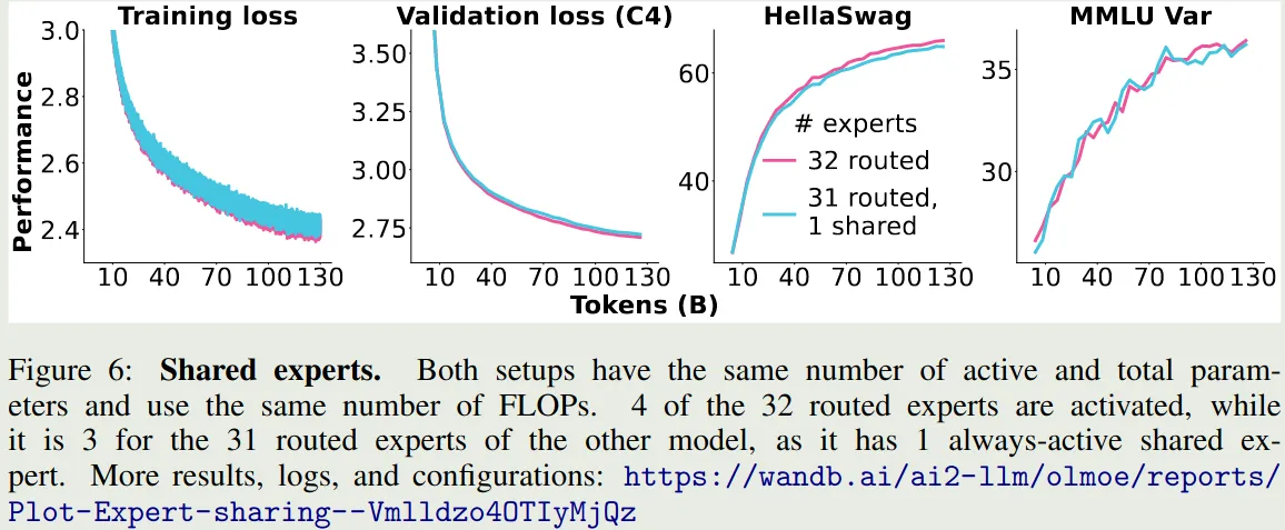
作者认为，加入 shared experts 之后，组合的可能性有所减少，这会降低模型的泛化性。因此，在 olmoe 中，作者没有使用 shared experts.

Ling-mini-beta (Tian et al., 2025) 通过实验得出的结论为，shared expert 应该是一个非零的尽可能小的值，作者认为将 shared expert 设置为 1 是一个比较合理的选择。

Activation Function

一般来说，在选取 top-K 专家时，我们会对 gating layer 的输出进行归一化，通常我们会使用 softmax function:

G(x) = \mathrm{softmax}(W_gx + b)\in\mathbb{R}^N

但是，在 Loss-Free Balancing 中，作者通过实验发现，使用 sigmoid 作为激活函数效果更好，即

G(x) = \mathrm{sigmoid}(W_gx + b)\in\mathbb{R}^N

其对应的实验结果如下图所示

最近的 DeepSeek-V4 (DeepSeek-AI, 2026) 使用了 $\mathrm{Sqrt}(\mathrm{Softplus}(\cdot))$ 作为激活函数。

实验结果显示，sigmoid function 对于超参数更加 robust, 且表现也更好一些。下面是一些使用不同激活函数的模型例子

Activation function	Models
$\mathrm{softmax}(\cdot)$	Step 3, Kimi-K2, gpt-oss-120B
$\mathrm{sigmoid}(\cdot)$	GLM-4.5, dots.llm1, DeepSeek-V3, MiniMax-M2
$\mathrm{Sqrt}(\mathrm{Softplus}(\cdot))$	DeepSeek-V4

Routing Z-loss

Routing Z-loss 由 ST-MoE (Zoph et al., 2022) 提出， Switch Transformer (Fedus et al., 2022) 发现在 gating layer 中使用 float32 精度可以提高训练稳定性，但是这还不够，因此 ST-MoE 使用了如下的 router Z-loss:

\mathcal{L}_z(x) = \frac1B\sum_{i=1}^B\left(\log\sum_{j=1}^N e^{x_j^{(i)}}\right)^2

其中 $B$ 是 batch size ， $x_j^{(i)}=[W_gx_i+b]_j$ 代表了第 $j$ 个专家对 $i$ 个 token 的激活 logits. OLMoE (Muennighoff et al., 2025) 实验验证结果如下

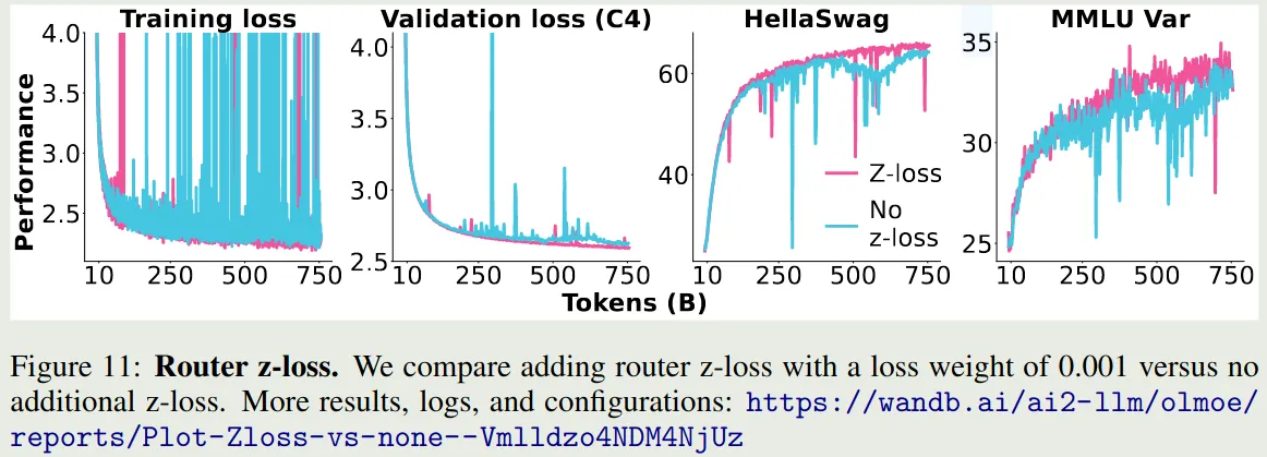
可以看到，加入 router Z-loss 之后，模型训练的稳定性有所提升，因此 Olmoe 采取了这个改进，但是后续的 MoE 模型使用 Z-loss 较少，个人猜测原因是 Loss-Free Balancing 中提出的加入额外的 loss 会影响 nex-token prediction loss

Routing Strategy

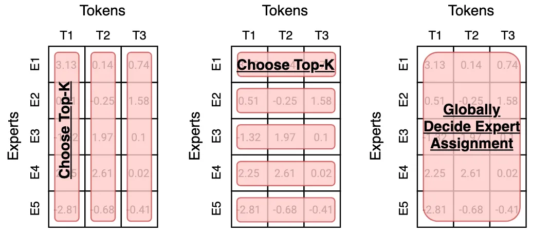
routing 策略直接决定了 MoE 模型的有效性。在为专家分配 token 的时候，我们有如下方式：

为每个 token 选取若干个专家
为每个专家选取若个个 token
动态分配 token 与专家之间的关系

三种选择方式如下图所示，图源 (Fedus, Dean, et al., 2022)

Expert Choice

每个专家选取 top-k 的 token，此时每个专家处理的 token 个数是相同的，这个方法的好处是自带 load balance。缺点是自回归生成的方式没有完整序列长度的信息，从而导致 token dropping，也就是某些 token 不会被任何专家处理，某些 token 会被多个专家处理。

目前采用这个策略的有 OpenMoE-2，核心思想是 dLLM 的输出长度固定，expert choice 策略更有效

Token Choice

每个 token 选取 top-k 的专家，好处是每个 token 都会被处理，缺点是容易导致负载不均衡。因此，一般需要加上负载均衡或者 token dropping 策略来提高负载均衡

Capacity Factor 由 Switch Transformer (Fedus, Zoph, et al., 2022) 提出，其定义为

\text{expert capacity} = \left(\frac{\text{tokens per batch}}{\text{number of experts}}\right) * \text{capacity factor}

设置 capacity factor 之后，当某个专家处理的 token 个数超过 capacity 之后，概专家的计算就会直接跳过，退化为 residual connection. 后续 DeepSeek-V2 (DeepSeek-AI et al., 2024) 也采用了这种策略，但是 DeepSeek-V3 (DeepSeek-AI et al., 2025) 弃用

Load balancing Loss 在训练目标中加入负载均衡损失，要求每个专家处理的 token 个数的分布尽可能均匀。这部分具体见 Loss-Free Balancing

Global Choice

全局分配决定 token 和专家的匹配关系，后续 Qwen 提出了 Global-batch load balancing 使用了这种方式来提高专家的特化程度

Dynamic Routing

根据输入 token 的难度动态决定激活专家的个数。LongCat-Flash (M. L. Team et al., 2025) 使用了一个 Phantom expert 的方法来实现根据 token 的难度动态分配专家。具体来说，除了 $N$ 个专家之外，MoE 还包括 $Z$ 个 zero-computation expert (现在一共有 $N+Z$ 个专家参与计算), 其计算方式如下

\begin{aligned} y &= \sum_{i=1}^{K}\mathrm{Normalize}(G_{e_i}) E_{e_i}(x), e_i \in \{i\mid G_i(x)\in \mathrm{TopK}(G_i(x), K)\}\\ E_{e_i}(x) &= \begin{cases} FFN_{e_i}(x), & \text{ if }1\leq i\leq N\\ x, & \text{ otherwise }\\ \end{cases} \end{aligned}

注：LongCat 还使用了 Loss-Free Balancing, 我们这里省略掉了。

Hash Routing

TODO, 最近的 DeepSeek-V4 (DeepSeek-AI, 2026) 在前三层 MoE layer 中使用了 Hash Routing 策略。

Overview

现在几乎所有的模型都选择方式 1，即每个 token 选取 top-k 的专家。 OLMoE (Muennighoff et al., 2025) 对比了以下方式 1 和方式 2 的表现，如下图所示

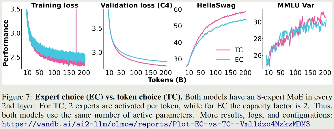
可以看到，加入 load balancing loss 之后，相比于 Expert Choice, Token Choice 的表现更好。但是，expert choice 更加高效，作者认为 expert choice 更适用于多模态，因为丢掉 noise image tokens 对 text token 影响会比较小。因此，在 OLMoE (Muennighoff et al., 2025) 中，作者使用 token choice 作为 routing 策略

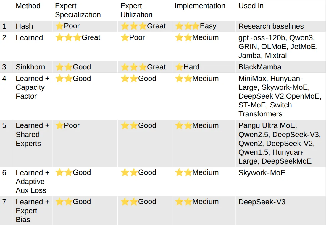
Routing strategy overview (Cerebras) — Credit to Celebras

Upcycling

upsampling 是一个将 dense model 转化为 MoEmodel 的方法，具体做法就是我们复制 dense model 中的 FFN layer 得到对应 MoE layer 中的 Expert，然后我们再结合 router 训练，这样可以提高整体的训练效率。相关模型有 MiniCPM (Hu et al., 2024), Qwen1.5 (Q. Team, 2024) 和 Mixtral MoE(Jiang et al., 2024) (疑似)

OLMoE (Muennighoff et al., 2025) 给出的实验结果如下图所示

从已有的结果来看，MoE 模型会被 dense 模型的一些超参数所限制，且训练不是很稳定。因此，现在一般不采用这种方法

Dai, D., Deng, C., Zhao, C., Xu, R. X., Gao, H., Chen, D., Li, J., Zeng, W., Yu, X., Wu, Y., Xie, Z., Li, Y. K., Huang, P., Luo, F., Ruan, C., Sui, Z., & Liang, W. (2024). DeepSeekMoE: Towards Ultimate Expert Specialization in Mixture-of-Experts Language Models. https://arxiv.org/abs/2401.06066 back: 1, 2, 3, 4, 5
DeepSeek-AI. (2026). DeepSeek-V4: Towards Highly Efficient Million-Token Context Intelligence. https://huggingface.co/deepseek-ai/DeepSeek-V4-Pro/blob/main/DeepSeek_V4.pdf back: 1, 2
DeepSeek-AI, Liu, A., Feng, B., Wang, B., Wang, B., Liu, B., Zhao, C., Dengr, C., Ruan, C., Dai, D., Guo, D., Yang, D., Chen, D., Ji, D., Li, E., Lin, F., Luo, F., Hao, G., Chen, G., … Xie, Z. (2024). DeepSeek-V2: A Strong, Economical, and Efficient Mixture-of-Experts Language Model. https://arxiv.org/abs/2405.04434
DeepSeek-AI, Liu, A., Feng, B., Xue, B., Wang, B., Wu, B., Lu, C., Zhao, C., Deng, C., Zhang, C., Ruan, C., Dai, D., Guo, D., Yang, D., Chen, D., Ji, D., Li, E., Lin, F., Dai, F., … Pan, Z. (2025). DeepSeek-V3 Technical Report. https://arxiv.org/abs/2412.19437 back: 1, 2, 3
Fedus, W., Dean, J., & Zoph, B. (2022). A Review of Sparse Expert Models in Deep Learning. https://arxiv.org/abs/2209.01667
Fedus, W., Zoph, B., & Shazeer, N. (2022). Switch transformers: scaling to trillion parameter models with simple and efficient sparsity. J. Mach. Learn. Res., 23(1). back: 1, 2, 3, 4
Hu, S., Tu, Y., Han, X., He, C., Cui, G., Long, X., Zheng, Z., Fang, Y., Huang, Y., Zhao, W., Zhang, X., Thai, Z. L., Zhang, K., Wang, C., Yao, Y., Zhao, C., Zhou, J., Cai, J., Zhai, Z., … Sun, M. (2024). MiniCPM: Unveiling the Potential of Small Language Models with Scalable Training Strategies. https://arxiv.org/abs/2404.06395
Jiang, A. Q., Sablayrolles, A., Roux, A., Mensch, A., Savary, B., Bamford, C., Chaplot, D. S., de las Casas, D., Hanna, E. B., Bressand, F., Lengyel, G., Bour, G., Lample, G., Lavaud, L. R., Saulnier, L., Lachaux, M.-A., Stock, P., Subramanian, S., Yang, S., … Sayed, W. E. (2024). Mixtral of Experts. https://arxiv.org/abs/2401.04088
MiniMax, :, Chen, A., Li, A., Zhou, B., Gong, B., Jiang, B., Dan, B., Yu, C., Wang, C., Ma, C., Zhong, C., Zhu, C., Xiao, C., Yang, C., Du, C., Zhang, C., Zhang, C., Huang, C., … Ge, Z. (2026). The MiniMax-M2 Series: Mini Activations Unleashing Max Real-World Intelligence. https://arxiv.org/abs/2605.26494
Muennighoff, N., Soldaini, L., Groeneveld, D., Lo, K., Morrison, J., Min, S., Shi, W., Walsh, E. P., Tafjord, O., Lambert, N., Gu, Y., Arora, S., Bhagia, A., Schwenk, D., Wadden, D., Wettig, A., Hui, B., Dettmers, T., Kiela, D., … Hajishirzi, H. (2025). OLMoE: Open Mixture-of-Experts Language Models. The Thirteenth International Conference on Learning Representations. https://openreview.net/forum?id=xXTkbTBmqq back: 1, 2, 3, 4, 5, 6
Qwen, :, Yang, A., Yang, B., Zhang, B., Hui, B., Zheng, B., Yu, B., Li, C., Liu, D., Huang, F., Wei, H., Lin, H., Yang, J., Tu, J., Zhang, J., Yang, J., Yang, J., Zhou, J., … Qiu, Z. (2025). Qwen2.5 Technical Report. https://arxiv.org/abs/2412.15115
Team, K., Bai, Y., Bao, Y., Charles, Y., Chen, C., Chen, G., Chen, H., Chen, H., Chen, J., Chen, N., Chen, R., Chen, Y., Chen, Y., Chen, Y., Chen, Z., Cui, J., Ding, H., Dong, M., Du, A., … Zu, X. (2026). Kimi K2: Open Agentic Intelligence. https://arxiv.org/abs/2507.20534
Team, M. L., Bayan, Li, B., Lei, B., Wang, B., Rong, B., Wang, C., Zhang, C., Gao, C., Zhang, C., Sun, C., Han, C., Xi, C., Zhang, C., Peng, C., Qin, C., Zhang, C., Chen, C., Wang, C., … Su, Z. (2025). LongCat-Flash Technical Report. https://arxiv.org/abs/2509.01322
Team, Q. (2024). Introducing Qwen1.5. https://qwen.ai/blog?id=qwen1.5 back: 1, 2
Tian, C., Chen, K., Liu, J., Liu, Z., Zhang, Z., & Zhou, J. (2025). Towards Greater Leverage: Scaling Laws for Efficient Mixture-of-Experts Language Models. https://arxiv.org/abs/2507.17702 back: 1, 2
Yang, A., Yang, B., Hui, B., Zheng, B., Yu, B., Zhou, C., Li, C., Li, C., Liu, D., Huang, F., Dong, G., Wei, H., Lin, H., Tang, J., Wang, J., Yang, J., Tu, J., Zhang, J., Ma, J., … Fan, Z. (2024). Qwen2 Technical Report. https://arxiv.org/abs/2407.10671
Zoph, B., Bello, I., Kumar, S., Du, N., Huang, Y., Dean, J., Shazeer, N., & Fedus, W. (2022). ST-MoE: Designing Stable and Transferable Sparse Expert Models. https://arxiv.org/abs/2202.08906

Load Balancing Loss

我们在 MoE Design 中已经介绍了 MoE 模块，MoE 尽管可以在相同的算力下扩大模型的 size, 但是其问题在于训练时容易出现负载不均衡，也就是说只有少数几个专家被激活，其他专家处于闲置状态，从而导致模型性能下降或者退化。

为了解决这个问题，一个通用的做法是使用 load balancing loss. load balancing loss 可以有效实现负载均衡，让各个专家被激活的概率差不多。

我们按照时间发展顺序来介绍 load balancing loss 的推导。

Derivation

我们假设输入的 batch size 为 $B$ , 总专家个数为 $N$ , 激活专家个数为 $K$ , $G_i(x_j)$ 代表 gating layer 预测的第 $i$ 个专家对于 token $x_j$ 的重要性程度。

第一个阶段的 load balancing loss 针对广义的 MoE 模型。 (Bengio et al., 2016) 提出了一个让 batch 里每个专家平均激活概率分布更均匀的损失函数，其定义如下所示

L_b = \sum_{i=1}^N\left\Vert \frac1B\sum_{j=1}^BG_i(x_j) - \frac1N\right\Vert_2

其主要目标是让每个专家的平均激活概率接近 $1/N$ , 即均匀分布.

(Shazeer et al., 2017) 对上面的损失函数进行了改进，提出了变异系数 $\mathrm{CV}(\cdot)$ 来保证负载均衡，其定义如下：

L_{importance} = \mathrm{CV}(\mathrm{Importance}(X))^2

这里

\mathrm{Importance}_i(X) = \sum_{j=1}^B G_i(x_j),\ \mathrm{CV}(X)= \frac{\mathrm{var}[X]}{\mathbb{E}[X]},\ i=1,\dots,N

注意到 $\mathrm{var}[X]\geq0$ , 当且仅当 $X$ 为均匀分布时 $\mathrm{var}[X]=0$ , 因此 important loss 可以让每个专家在一个 batch 中的激活的平均概率尽可能一致。

但是平均概率一致不代表各个专家处理的 token 个数一致，比如一个专家可能处理比较少的 token, 但是每个 token 的权重都很大。为了解决这个问题，作者额外加入了 load balancing loss

\mathcal{L}_{\mathrm{load}} = \mathrm{CV}(\mathrm{Load}(X))^2

其中

\begin{aligned} \mathrm{Load}_i(X) &= \mathrm{soft\_estimation}\left(\sum_{j=1}^B\mathbb{1}(\text{token }j \text{ selects expert }i)\right)\\ &=\mathrm{soft\_estimation}\left(\sum_{j=1}^B\mathbb{1}\{i\in\mathrm{TopK}(\{G_i(x_j)\}_{i=1}^{E}, K)\}\right),\ i=1,\dots,N \end{aligned}

这里 $\mathrm{soft\_estimation}$ 是作者针对离散变量进行的一个光滑化处理，以方便反向传播。

GShard (Lepikhin et al., 2021) 进一步对 (Shazeer et al., 2017) 提出的 loss 进行了简化，首先注意到 $\sum_{i=1}^N\mathrm{Load}_i(X)=BK$ , 因此我们有

\begin{aligned} \mathcal{L}_{\mathrm{load}} &= \mathrm{CV}(\mathrm{Load}(X))^2 \\ &= \left(\frac{\mathrm{var}[\mathrm{Load}(X)]}{\mathbb{E}[\mathrm{Load}(X)]}\right)^2\\ &= \left(C_1[\mathrm{Load}(X)]\right)^2\\ &= C_1\mathbb{E}[\mathrm{Load}(X)^2]-C_2 \end{aligned}

这里 $C_1,C_2$ 均为常数。GShard 并没有使用 soft estimation, 因此这里的 $\mathrm{Load}_i(X)$ 定义为

\mathrm{Load}_i(X)=\sum_{j=1}^B\mathbb{1}(\text{token }j \text{ selects expert }i),\ i=1,\dots,N

其代表了 一个 batch 里专家 $i$ 被激活的次数，理想情况下，所有专家被激活的次数应该是一致的，从而我们就实现了负载均衡。

但是现在的问题是， $\mathrm{Load}_i(X)$ 是一个离散变量，为了解决这个问题，作者使用了重要性来进行近似，即

\mathcal{L}_{\mathrm{load}} = \mathbb{E}[\mathrm{Load}(X)^2]\approx \mathbb{E}[\mathrm{Load}(X)\cdot\mathrm{Importance}(X)]

Switch Transformer (Fedus et al., 2022) 又对 GShard (Lepikhin et al., 2021) 提出的 load balancing loss 进行了规范化，这也是现在大部分 load balancing loss 使用的形式，其定义如下：

\mathcal{L}_{\mathrm{load}} = \sum_{i=1}^N f_i P_i

其中，

f_i = \frac{1}{B}\mathrm{Load}_i(X)=\frac{1}{B}\sum_{j=1}^B\mathbb{1}(\text{token }j \text{ selects expert }i),\ i=1,\dots,N

代表了分配给专家 $i$ 的 token 比例，

P_i = \frac{1}{B}\mathrm{Importance}_i(X) = \frac{1}{B}\sum_{j=1}^B G_i(x_j)

代表了这个 batch 里专家 $i$ 的平均激活概率。我们可以看到，这个形式和 GShard (Lepikhin et al., 2021) 实际上是等价的：

\mathcal{L}_{\mathrm{load}} = \sum_{i=1}^N f_i P_i = \mathbb{E}[\mathbf{f}\cdot \mathbf{P}] = N \mathbb{E}[\mathrm{Load}(X)\cdot\mathrm{Importance}(X)]

Analysis

目前关于 load balancing loss 可以实现负载均衡的数学分析是比较少的。Switch Transformer (Fedus et al., 2022) 中进行了如下分析：

The auxiliary loss of Equation 4 encourages uniform routing since it is minimized under a uniform distribution.

Switch Transformer

但实际上，这个分析是错误的，Switch transformer 中定义的 load balancing loss 并不是在均匀分布时取最小值，而是取最大值。考虑如下情形，

\mathbf{f}=[1,\dots,0],\ \mathbf{P}=[0,\dots,1]

此时，我们有

\mathbf{f}\cdot \mathbf{P} = 0\leq [1/N,\dots,1/N]\cdot [1/N,\dots,1/N] = 1/N.

我找了很多资料，最后发现苏剑林老师在 (苏剑林, 2025) 中进行了分析。我这里基于苏剑林老师的 blog 进行了一下总结。

分析的核心思想就是，尽管 load balancing loss 目标函数没有意义，但是我们通过 straight-through estimator (STE)，就可以得到一个有意义的目标函数，其梯度与 load balancing loss 目标函数的梯度是一致的，这样 load balancing loss 目标函数就完成了其负载均衡的目标。

注意到 load balancing loss 的最终目标是让每个专家处理的 token 个数尽可能一致，也就是

\mathcal{L}_{\mathrm{load}} = \sum_{j=1}^B \left(f_i-\frac1B\right)^2

但是 $f_i=\mathrm{Load}_i(X)$ 是一个离散变量不可导，因此，基于 STE, 我们可以将其改写为

\mathcal{L}_{\mathrm{load}} = \sum_{j=1}^B \left(P_i+\mathrm{sg}[f_i-P_i]-\frac1B\right)^2

其中 $\mathrm{sg}[\cdot]$ 满足：

\mathrm{sg}[\cdot]=\begin{cases} x, &\text{forward pass}\\ 0, &\text{backward pass} \end{cases}

此时我们目标函数的梯度就变成了

\begin{aligned} \nabla_\theta\mathcal{L}_{\mathrm{load}} &= \sum_{j=1}^B 2\nabla_\theta\left(P_i+\mathrm{sg}[f_i-P_i]-\frac1B\right)\left(P_i+\mathrm{sg}[f_i-P_i]-\frac1B\right)\\ &= 2\sum_{j=1}^B\nabla_\theta P_i\left(f_i-\frac1B\right)\\ &= 2\sum_{j=1}^B\nabla_\theta P_i\left(f_i-\frac1B\right)\\ &= 2\nabla_\theta \left(\sum_{j=1}^Bf_iP_i\right) \end{aligned}

这样就对应上了我们之前的目标函数。总之，目标函数尽管本身没有意义，但是其对应的梯度却可以让模型实现负载均衡的目标。

Extension

Loss Free Load Balancing Strategy

Loss-Free load balancing (Wang et al., 2024) 是 DeepSeek 提出来的一个无需 load balancing loss 实现负载均衡的方法。其核心思想是 load balancing loss 会影响语言建模性能，因此在 $\mathrm{TopK}$ 操作时，作者加入一些扰动，从而让负载高的专家被选择的概率降低，让负载低的专家被选择的概率提高。

具体做法就是在每个专家的 gating score 上加入一个 bias term, 然后再决定对应的专家：

g_{i,t} = \begin{cases} s_{i,t}, & s_{i,t}+b_i\in\mathrm{Topk}(\{s_{i,j}+b_j\mid 1\leq j\leq N\}, K)\\ 0, &\text{otherwise} \end{cases}

注意这里的 bias item 仅影响 top-K 操作，其对最终的输出没有影响。

为了实现负载均衡，作者根据上一个 batch 的 expert load 情况来调整 bias item, 如果某一个专家的 load 太大，则对应的 bias item 会变小。其算法实现过程如下：

Algorithm: Adjusting the per-expert bias during training

Input: MoE model $\theta$ , training batch iterator $B$ , bias update rate $u$

Initialize $b_i=0$ for each expert

For a batch $\{(x_k,y_k)\}\in B$

Train MoE model $\theta$ on the batch data $\{(x_k,y_k)\}$ , with gating score calculated
Count the number of assigned tokens $c_i$ for each expert, and the average number $\bar{c}_i$
Calculate the load violation error $e_i=\bar{c}_i=c_i$
Update $b_i$ by $b_i=b_i+u*\mathrm{sign}(e_i)$

Return trained model $\theta$ , corresponding bias $b_i$

作者对比不同的负载均衡算法如下表所示

Load Balancing Methods	Balanced Expert Load	Interference Gradients	Future Token Leakage
Loss-Controlled (strong auxiliary loss)	balanced	strong	no leakage
Loss-Controlled (weak auxiliary loss)	imbalanced	weak	no leakage
Expert Choice	balanced	none	with leakage
Loss-Free (Ours)	balanced	none	no leakage

TODO

Global-batch Load Balancing Loss Strategy

Global-batch Load Balancing (Qiu et al., 2025) 是 Qwen 提出来的一个提高负载均衡的方法。其核心思想是，现有的 token choice 只是在 batch 层面达到负载均衡，这种局部均衡的性质可能会对模型的全局均衡性产生影响。因此，作者就预先在 global batch 层面对专家进行分配，从而提高专家在不同 domain 上的特化程度。

一般来说，MoE 模型训练时会使用 expert parallel 策略，此时 load balancing loss 修改为

\mathrm{LBL}_{\mathrm{micro}}= \frac{1}{N_P}\sum_{j=1}^{N_P}\left(N_E\sum_{i=1}^{N_E}f_i^hP_i^j\right)

其中 $N_P$ 是 parallel groups 的个数。在这种情况下，模型需要再每个 parallel group 中实现负载均衡。但是某一个 mircro-batch 里可能只包含某一个 domain 的序列，因此各个专家被强制要求在每一个 domain 中也均衡分布。作者认为，这种方式会限制专家的能力，进而影响模型的表现。

作者的解决方法在于，获取每个 parallel group 的 $f_i$ 然后求 global-batch 的 $\bar{f}_i$ .

\mathrm{LBL}_{\mathrm{global}}=N_E\sum_{i=1}^{N_E}\bar{f}_i\bar{P}_i=N_E\sum_{i=1}^{N_E}\bar{f}_i\left(\frac{1}{N_P}\sum_{j=1}^{N_P}P_j\right) = \frac{1}{N_P}\sum_{j=1}^{N_P}\left(N_E\sum_{i=1}^{N_E}\bar{f}_iP_i^j\right)

实际中，由于计算节点数量有限，micro-batch size 之和可能会小于 global-batch size, 因此我们会使用 gradient accumulation. 在这种情况下，作者使用了一个 buffer 来保存多个 micro-batch 的专家选择次数，最终算法实现过程如下所示

Algorithm: Approximate Global-Batch LBL

Initialize an empty buffer for each expert $c_i=0$

While training continues

For each gradient accumulation step
- Add $c_i$ with new synchtonized selection counts for expert $i$
- Calculate the current $f_i$ with $c_i$ , $i\in N_E$ in the buffer
Optimizer step, clear gradient
Reset the buffer with $c_i=0$

Sequence level load balancing loss

TODO

Node level load balancing loss

TODO

Experiments

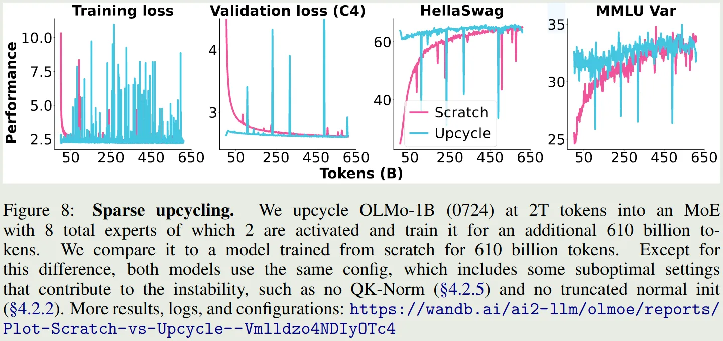
OLMoE (Muennighoff et al., 2025) 对比了加入 load balancing loss 之后模型的表现变化情况，结果如下图所示

可以看到，加入 load balancing loss 之后，模型的表现均超过了不加时的表现。

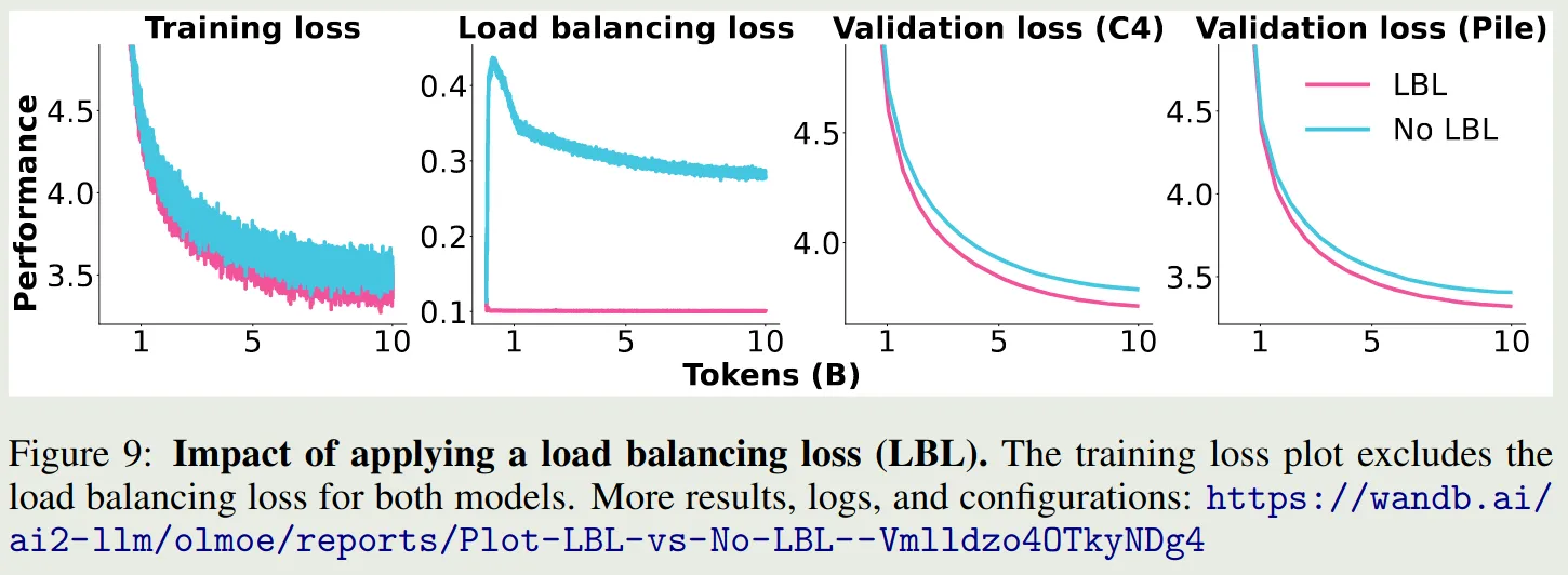
作者进一步分析了不同专家在加/不加 load balancing loss 时的激活情况，结果如下图所示

visualization of expert assignment on load balancing

结果显示，load balancing loss 确实可以让不同专家的激活概率大致相当。

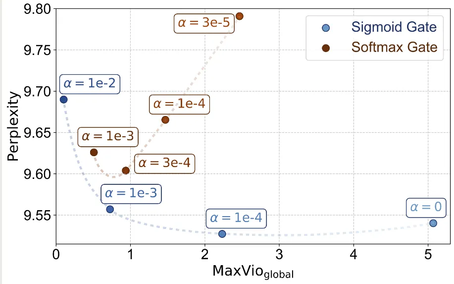
(Wang et al., 2024) 使用了 DeepSeekMoE 来进行实验，作者使用了 sigmoid function 作为 gating function, 因为作者发现 sigmoid function 效果比 softmax 效果更好。

作者提出了 maximal violation (MaxVio) 来量化一个 MoE layer 的负载均衡程度

\mathrm{MaxVio} = \frac{\max_i\mathrm{Load}_i-\overline{\mathrm{Load}_i}}{\overline{\mathrm{Load}_i}}

其中 $\mathrm{Load}_i$ 代表了分配给第 $i$ 个专家的 token 个数， $\overline{\mathrm{Load}_i}$ 代表了理想情况下的负载均衡。

实验结果如下图所示

Model Size	Load Balancing Methods	Validation Perplexity	MaxVio_global
1B	Loss-Controlled	9.56	0.72
1B	Loss-Free	9.50	0.04
3B	Loss-Controlled	7.97	0.52
3B	Loss-Free	7.92	0.04

实验结果显示，本文提出的 Loss-Free Balancing 效果更好，且负载均衡更高

Bengio, E., Bacon, P.-L., Pineau, J., & Precup, D. (2016). Conditional Computation in Neural Networks for faster models. https://arxiv.org/abs/1511.06297
Fedus, W., Zoph, B., & Shazeer, N. (2022). Switch transformers: scaling to trillion parameter models with simple and efficient sparsity. J. Mach. Learn. Res., 23(1). back: 1, 2
Lepikhin, D., Lee, H., Xu, Y., Chen, D., Firat, O., Huang, Y., Krikun, M., Shazeer, N., & Chen, Z. (2021). Ghard: Scaling Giant Models with Conditional Computation and Automatic Sharding. International Conference on Learning Representations. https://openreview.net/forum?id=qrwe7XHTmYb back: 1, 2, 3
Muennighoff, N., Soldaini, L., Groeneveld, D., Lo, K., Morrison, J., Min, S., Shi, W., Walsh, E. P., Tafjord, O., Lambert, N., Gu, Y., Arora, S., Bhagia, A., Schwenk, D., Wadden, D., Wettig, A., Hui, B., Dettmers, T., Kiela, D., … Hajishirzi, H. (2025). OLMoE: Open Mixture-of-Experts Language Models. The Thirteenth International Conference on Learning Representations. https://openreview.net/forum?id=xXTkbTBmqq
Qiu, Z., Huang, Z., Zheng, B., Wen, K., Wang, Z., Men, R., Titov, I., Liu, D., Zhou, J., & Lin, J. (2025). Demons in the Detail: On Implementing Load Balancing Loss for Training Specialized Mixture-of-Expert Models. https://arxiv.org/abs/2501.11873
Shazeer, N., Mirhoseini, *Azalia, Maziarz, *Krzysztof, Davis, A., Le, Q., Hinton, G., & Dean, J. (2017). Outrageously Large Neural Networks: The Sparsely-Gated Mixture-of-Experts Layer. International Conference on Learning Representations. https://openreview.net/forum?id=B1ckMDqlg back: 1, 2
Wang, L., Gao, H., Zhao, C., Sun, X., & Dai, D. (2024). Auxiliary-Loss-Free Load Balancing Strategy for Mixture-of-Experts. https://arxiv.org/abs/2408.15664 back: 1, 2
苏剑林. (2025, February). MoE环游记：2、不患寡而患不均. %5Curl%7Bhttps://spaces.ac.cn/archives/10735%7D

Analysis on MoE

前面的章节我们介绍了 MoE layer design 和如何通过 load balancing loss 来提高 MoE 的负载均衡。这一节我们来分析一下 MoE layer 的性质。

Specialization of Experts

OpenMoE (Xue et al., 2024) 分析了 MoE 模型的特化程度，其结论如下

大部分专家对于不同的 domain 没有出现 specialization 情况，对于 math domain, specialization 现象比较明显，作者认为这是因为 math domain 包含更多的 special tokens
部分专家对于 position ID 有 specialization 现象，并且连续的 token 更偏好相同的专家
部分专家对于 Token ID 有 specialization 现象，作者将这种现象称为 Context-independent Specialization.
专家还会对语义相似的 token 进行聚类，并且这种聚类在训练早期就已经发生，作者认为其原因在于重新分配 token 会增加最终的 loss
对于 token dropping, 作者发现越靠后的 token, 其被 drop 的概率比例也越高。并且对于指令跟随数据，更多的 token 都会被丢掉，因此作者认为指令跟随数据是 MoE 模型的一种 OOD 数据

Saturation of Experts

OLMoE (Muennighoff et al., 2025) 探究了训练过程中激活的专家和训练结束后激活的专家的匹配程度，结果如下图所示

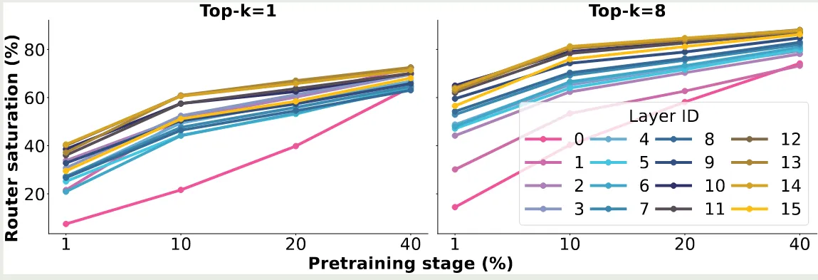
实验结果说明，训练 $1\%$ 的数据之后，就有 $40\%$ 的 routing 和训练完毕的 routing 一致，当训练 $40\%$ 的数据之后，这个比例提升到了 $80\%$ . 作者认为，这是专家特化的结果，初始的 routing 如果改变的话会带来表现下降，因此模型倾向于使用固定的专家处理特定的 token

作者还发现，later layers 比 early layers 饱和更快，early layer, 特别是 layer 0, 饱和的非常慢。作者认为，这是 DeepSeekMoE (Dai et al., 2024) 放弃在第一层使用 MoE layer 的原因，因为 load balancing loss 收敛更慢。后续 DeepSeek-V2 (DeepSeek-AI et al., 2024) 和 DeepSeek-V3 (DeepSeek-AI et al., 2025) 均在 early layer 上使用 dense layer 替换掉了 MoE layer

Dai, D., Deng, C., Zhao, C., Xu, R. X., Gao, H., Chen, D., Li, J., Zeng, W., Yu, X., Wu, Y., Xie, Z., Li, Y. K., Huang, P., Luo, F., Ruan, C., Sui, Z., & Liang, W. (2024). DeepSeekMoE: Towards Ultimate Expert Specialization in Mixture-of-Experts Language Models. https://arxiv.org/abs/2401.06066
DeepSeek-AI, Liu, A., Feng, B., Wang, B., Wang, B., Liu, B., Zhao, C., Dengr, C., Ruan, C., Dai, D., Guo, D., Yang, D., Chen, D., Ji, D., Li, E., Lin, F., Luo, F., Hao, G., Chen, G., … Xie, Z. (2024). DeepSeek-V2: A Strong, Economical, and Efficient Mixture-of-Experts Language Model. https://arxiv.org/abs/2405.04434
DeepSeek-AI, Liu, A., Feng, B., Xue, B., Wang, B., Wu, B., Lu, C., Zhao, C., Deng, C., Zhang, C., Ruan, C., Dai, D., Guo, D., Yang, D., Chen, D., Ji, D., Li, E., Lin, F., Dai, F., … Pan, Z. (2025). DeepSeek-V3 Technical Report. https://arxiv.org/abs/2412.19437
Muennighoff, N., Soldaini, L., Groeneveld, D., Lo, K., Morrison, J., Min, S., Shi, W., Walsh, E. P., Tafjord, O., Lambert, N., Gu, Y., Arora, S., Bhagia, A., Schwenk, D., Wadden, D., Wettig, A., Hui, B., Dettmers, T., Kiela, D., … Hajishirzi, H. (2025). OLMoE: Open Mixture-of-Experts Language Models. The Thirteenth International Conference on Learning Representations. https://openreview.net/forum?id=xXTkbTBmqq
Xue, F., Zheng, Z., Fu, Y., Ni, J., Zheng, Z., Zhou, W., & You, Y. (2024). OpenMoE: An Early Effort on Open Mixture-of-Experts Language Models. https://arxiv.org/abs/2402.01739

Optimization

MoE 模型的优势在于表现好，但是模型参数往往非常大，为了方便使用，我们需要对训练好的 MoE 模型进行优化，目前主要有蒸馏，专家剪枝/合并以及量化等优化方法

蒸馏是一个将大模型能力传递给小模型的做法，目前已有的包括：

Switch Transformer (Fedus et al., 2022) 通过蒸馏，在仅使用 $1/20$ 参数的情况下，保留了稀疏教师模型 $30\%$ 的表现
Gemini 2.5 (Comanici et al., 2025) 通过蒸馏 Gemini2.5 Pro 得到 Gemini2.5 Flash
DeepSeek-R1 (Guo et al., 2025) 通过蒸馏来提升小语言模型的 reasoning 能力
Qwen3 (Yang et al., 2025) 对于小语言模型的训练使用了 off-policy distillation 和 on-policy distillation 来训练小语言模型

Comanici, G., Bieber, E., Schaekermann, M., Pasupat, I., Sachdeva, N., Dhillon, I., Blistein, M., Ram, O., Zhang, D., Rosen, E., Marris, L., Petulla, S., Gaffney, C., Aharoni, A., Lintz, N., Pais, T. C., Jacobsson, H., Szpektor, I., Jiang, N.-J., … Helmholz, W. (2025). Gemini 2.5: Pushing the Frontier with Advanced Reasoning, Multimodality, Long Context, and Next Generation Agentic Capabilities. https://arxiv.org/abs/2507.06261
Fedus, W., Zoph, B., & Shazeer, N. (2022). Switch transformers: scaling to trillion parameter models with simple and efficient sparsity. J. Mach. Learn. Res., 23(1).
Guo, D., Yang, D., Zhang, H., Song, J., Wang, P., Zhu, Q., Xu, R., Zhang, R., Ma, S., Bi, X., Zhang, X., Yu, X., Wu, Y., Wu, Z. F., Gou, Z., Shao, Z., Li, Z., Gao, Z., Liu, A., … Zhang, Z. (2025). DeepSeek-R1 incentivizes reasoning in LLMs through reinforcement learning. Nature, 645(8081), 633–638. 10.1038/s41586-025-09422-z
Yang, A., Li, A., Yang, B., Zhang, B., Hui, B., Zheng, B., Yu, B., Gao, C., Huang, C., Lv, C., Zheng, C., Liu, D., Zhou, F., Huang, F., Hu, F., Ge, H., Wei, H., Lin, H., Tang, J., … Qiu, Z. (2025). Qwen3 Technical Report. https://arxiv.org/abs/2505.09388

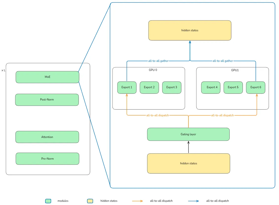
Infra

针对 MoE 模型的 infra 主要涉及 expert parallelism (EP), EP 将 MoE layer 的计算分为了三个阶段：

all-to-all dispatch: 基于 gating layer 的结果，将 token 通信传输到对应专家所在的 GPU 上
computation: 执行计算，即 $E_i(x)$ .
all-to-all combine: 收集专家计算的结果，即 $y = \sum_{i=1}^K\mathrm{Normalize}(G_{e_i}(x)) E_{e_i}(x)$ .

其框架图如下所示

Info on MoE models

MoE model information

Model	Year	total parameters	activated parameters	shared expert	Routed experts	activated experts
ST-MoE	2022/4	269B	32B	0	64	2
Mistral	2024/1	47B	13B	0	8	2
DeepSeek-MoE	2024/1	145B	22B	4	128	12
DeepSeek-V2	2024/5	236B	21B	2	160	6
LLaMA4	2025/4	400B	17B	1	128	1
DeepSeek-V3	2024/12	671B	37B	1	256	8
Qwen3	2025/5	235B	22B	0	128	8
dots.llm1	2025/6	142B	14B	2	128	6
Step 3	2025/7	316B	38B	1	48	3
Kimi-K2	2025/7	1043B	32B	8	384	1
GLM-4.5	2025/8	355B	32B	1	160	8
gpt-oss	2025/8	116B	5B	0	128	4
LongCat	2025/9	560B	27B*	0	768*	12
Ling-1T	2025/10	1000B	51B	1	256	8