Introduction
What is Distributed Training
分布式系统允许一个软件的多个组件运行在不同的机器上。与传统集中式系统不一样,分布式系统可以有效提高系统的稳健性。
一个比较比较经典的分布式就是 Git,Git 允许我们把代码保存在多个 remote 上。这样当一个 remote 宕机时,其他 remote 也能提供服务。
评估一个分布式系统的重要标准就是规模效益 (scalablity),也就是说,我们希望使用 8 台设备应该要比 4 台设备快 2 倍。 但是,由于通信带宽等原因,实际上加速比并不是和设备数量成线性关系。因此,我们需要设计分布式算法,来有效提高分布式系统的效率。
Why Distributed Training
我们需要分布式训练的原因主要是以下几点:
- 模型越来越大。当下(2025)领先模型如 Qwen,LLaMA 系列的最大模型都超过了 100B [2][3]。LLaMA 系列最大的模型甚至超过了 1000B。Scaling law 告诉我们模型表现与参数量,算力,数据量成正相关关系。
- 数据集越来越大。现在领先的模型需要的数据量基本都需要 100M 以上,而大语言模型训练需要的 token 数量也都超过了 10T 的量级 [2][3].
- 算力越来越强。现有最强的 GPU H100 其显存为 80GB,拥有 3.35TB/s 的带宽 (PcIe),这让训练大规模模型成为可能。
超大的模型使得我们很难在一张 GPU 上进行训练,甚至我们都很难使用单张 GPU 进行部署。 而 10T 级的数据也也需要几个月的时间才能训练完毕。 因此,如何高效利用多张 GPU 在大规模数据上训练超大模型就是我们需要解决的问题。
Notation
我们先来熟悉一下分布式训练中的一些基本概念:
- Host: host (master address) 是分布式训练中通信网络的主设备 (main device). 一般我们需要对其进行初始化
- Node: 一个物理或虚拟的计算单元,可以是一台机器,一个容器或者一个虚拟机
- Port: port (master port) 主要是用于通信的 master port
- Rank: rank 是通信网络中每个设备唯一的 ID
- world size: world size 是通信网络中设备的数量
- process group: 一个 process group 是通信网络中所有设备集合的一个子集。通过 process group, 我们可以限制 device 只在 group 内部进行通信
我们以下图为例:
上图中一共包含 2 个 node (2 台机器),每台机器包含 4 个 GPU (device),当我们初始化分布式环境时,我们一共启动了 8 个进程(每台机器 4 个进程),每个进程绑定一个 GPU.
在初始化分布式环境之间,我们需要指定 host 和 port。假设我们指定 host 为 node 0 和 port 为 29500,接下来,所有的进程都会基于这个 host 和 port 来与其他进程连接。
默认的 process group(包含所有 device)的 world size 为 8.
其细节展示如下
| process ID | rank | Node index | GPU index |
|---|---|---|---|
| 0 | 0 | 0 | 0 |
| 1 | 1 | 0 | 1 |
| 2 | 2 | 0 | 2 |
| 3 | 3 | 0 | 3 |
| 4 | 4 | 1 | 0 |
| 5 | 5 | 1 | 1 |
| 6 | 6 | 1 | 2 |
| 7 | 7 | 1 | 3 |
我们可以创建一个新的 process group,使其仅包含 ID 为偶数的 process:
| process ID | rank | Node index | GPU index |
|---|---|---|---|
| 0 | 0 | 0 | 0 |
| 2 | 1 | 0 | 2 |
| 4 | 2 | 1 | 0 |
| 6 | 3 | 1 | 2 |
Remark: 注意,rank 与 process group 相关,一个 process 在不同的 process group 里可能会有不同的 rank.
Single Node Training
TODO
Communication Primitives
接下来,我们需要介绍一下设备间的通信方式,这是我们后面分布式训练算法的基础。根据设备数量的不同,我们可以将设备间通信分为:
- one-to-one: 两个device之间互相进行通信
- one-to-many: 一个device与多个device进行通信
- many-to-one: 多个device与一个device之间进行通信
- many-to-many: 多个device之间互相进行通信
对应的示意图如下所示
One-to-one
One-to-one的情况很简单,一个 process 与另一个 process 进行通信,通信通过 send 和 recv 完成。
Send and Receive
测试代码如下:
An example of send and recv
# send_recv.py
import os

import torch
import torch.distributed as dist


def init_process():
    dist.init_process_group(backend='nccl')
    torch.cuda.set_device(dist.get_rank())

def example_send():
    if dist.get_rank() == 0:
        tensor = torch.tensor([1, 2, 3, 4, 5], dtype=torch.float32).cuda()
        dist.send(tensor, dst=1)
    elif dist.get_rank() == 1:
        tensor = torch.zeros(5, dtype=torch.float32).cuda()
        print(f"Before send on rank {dist.get_rank()}: {tensor}")
        dist.recv(tensor, src=0)
        print(f"After send on rank {dist.get_rank()}: {tensor}")


init_process()
example_send()

# run with
# torchrun --nproc_per_node=2 send_recv.py
Before send on rank 1: tensor([0., 0., 0., 0., 0.], device=‘cuda:1’)
After send on rank 1: tensor([1., 2., 3., 4., 5.], device=‘cuda:1’)
结果输出
注:为了方便,后续代码仅定义函数和运行方式,
init_process()和import部分省略
Isend and Irecev
send 和 recv 还有对应的 immediate 版本,即 isend 和 irecv,
send/recv的特点是在完成通信之前,两个 process 是锁住的。
与之相反,isend/irecv 则不会加锁,代码会继续执行然后返回 Work 对象,为了让通信顺利进行,我们可以在返回之前加入 wait()
An example of isend and irecv
# isend_irecv.py
def example_isend():
    req = None
    if dist.get_rank() == 0:
        tensor = torch.tensor([1, 2, 3, 4, 5], dtype=torch.float32).cuda()
        req = dist.isend(tensor, dst=1)
        print("Rank 0 is sending")

    elif dist.get_rank() == 1:
        tensor = torch.zeros(5, dtype=torch.float32).cuda()
        print(f"Before irecv on rank {dist.get_rank()}: {tensor}")
        req = dist.irecv(tensor, src=0)
        print("Rank 1 is receiving")
        req.wait()
        print(f"After isend on rank {dist.get_rank()}: {tensor}")

init_process()
example_isend()

# run with
# torchrun --nproc_per_node=2 isend_irecv.py
Before irecv on rank 1: tensor([0., 0., 0., 0., 0.], device=‘cuda:1’)
Rank 0 is sending
Rank 1 is receiving
After isend on rank 1: tensor([1., 2., 3., 4., 5.], device=‘cuda:1’)
由于isend/irecv这种不锁的特性,我们不应该
- 在
dist.isend()之前修改发送的内容tensor - 在
dist.irecv()之后读取接受的内容tensor
req.wait() 可以保证这次通信顺利完成,因此我们可以在req.wait()之后再进行修改和读取。
One-to-many
One-to-many 情形下,可以分为两种:scatter 和 broadcast
Scatter 的作用是将一个 process 的数据均分并散布到其他 process, Broadcast 的作用是将一个 process 的数据广播到其他 process. 两者不同的地方在于其他 process 获取到的是全量数据 (copy) 还是部分数据 (slice),其示意图如下所示
Scatter
Scatter 表达式为
Scatter 测试代码:
An example of scatter
# scatter.py
def example_scatter():
    if dist.get_rank() == 0:
        scatter_list = [
            torch.tensor([i+1] * 5, dtype=torch.float32).cuda()
            for i in range(dist.get_world_size())
        ]
        print(f"Rank 0 scatter list: {scatter_list}")
    else:
        scatter_list = None

    tensor = torch.zeros(5, dtype=torch.float32).cuda()
    print(f"Before scatter on rank {dist.get_rank()}: {tensor}")
    dist.scatter(tensor, scatter_list, src=0)
    print(f"After scatter on rank {dist.get_rank()}: {tensor}")

init_process()
example_broadcast()

# run with
# torchrun --nproc_per_node=4 broadcast.py
Rank 0 scatter list: [
tensor([1., 1., 1., 1., 1.], device=‘cuda:0’),
tensor([2., 2., 2., 2., 2.], device=‘cuda:0’),
tensor([3., 3., 3., 3., 3.], device=‘cuda:0’),
tensor([4., 4., 4., 4., 4.], device=‘cuda:0’)
]
Before scatter on rank 2: tensor([0., 0., 0., 0., 0.], device=‘cuda:2’)
Before scatter on rank 1: tensor([0., 0., 0., 0., 0.], device=‘cuda:1’)
Before scatter on rank 3: tensor([0., 0., 0., 0., 0.], device=‘cuda:3’)
Before scatter on rank 0: tensor([0., 0., 0., 0., 0.], device=‘cuda:0’)
After scatter on rank 0: tensor([1., 1., 1., 1., 1.], device=‘cuda:0’)
After scatter on rank 2: tensor([3., 3., 3., 3., 3.], device=‘cuda:2’)
After scatter on rank 3: tensor([4., 4., 4., 4., 4.], device=‘cuda:3’)
After scatter on rank 1: tensor([2., 2., 2., 2., 2.], device=‘cuda:1’)
Broadcast
Broadcast 的表达式为
Broadcast 测试代码:
An example of broadcast
# broadcast.py
def example_broadcast():
    if dist.get_rank() == 0:
        tensor = torch.tensor([1, 2, 3, 4, 5], dtype=torch.float32).cuda()
    else:
        tensor = torch.zeros(5, dtype=torch.float32).cuda()
    print(f"Before broadcast on rank {dist.get_rank()}: {tensor}")
    dist.broadcast(tensor, src=0)
    print(f"After broadcast on rank {dist.get_rank()}: {tensor}")


init_process()
example_broadcast()

# run with
# torchrun --nproc_per_node=3 broadcast.py
结果输出:
Before broadcast on rank 1: tensor([0., 0., 0., 0., 0.], device=‘cuda:1’)
Before broadcast on rank 2: tensor([0., 0., 0., 0., 0.], device=‘cuda:2’)
Before broadcast on rank 0: tensor([1., 2., 3., 4., 5.], device=‘cuda:0’)
After broadcast on rank 0: tensor([1., 2., 3., 4., 5.], device=‘cuda:0’)
After broadcast on rank 1: tensor([1., 2., 3., 4., 5.], device=‘cuda:1’)
After broadcast on rank 2: tensor([1., 2., 3., 4., 5.], device=‘cuda:2’)
Many-to-one
Many-to-one 情形下,也可以分为两种:gather 和 reduce.
Gather
Gather 对应 one-to-many 的 scatter 操作,负责将多个 process 的内容汇聚到一起,形成一个完整的向量,对应的表达式如下
示意图如下所示
测试代码如下
An example of gather
# gather.py
def example_gather():
    tensor = torch.tensor([dist.get_rank() + 1] * 5, dtype=torch.float32).cuda()
    if dist.get_rank() == 0:
        gather_list = [
            torch.zeros(5, dtype=torch.float32).cuda()
            for _ in range(dist.get_world_size())
        ]
        print(f"Rank 0 gather list: {gather_list}")
    else:
        gather_list = None

    print(f"Before gather on rank {dist.get_rank()}: {tensor}")
    dist.gather(tensor, gather_list, dst=0)
    if dist.get_rank() == 0:
        print(f"After gather on rank {dist.get_rank()}: {gather_list}")

init_process()
example_gather()

# run with
# torchrun --nproc_per_node=4 gather.py
Before gather on rank 3: tensor([4., 4., 4., 4., 4.], device=‘cuda:3’)
Before gather on rank 2: tensor([3., 3., 3., 3., 3.], device=‘cuda:2’)
Before gather on rank 0: tensor([1., 1., 1., 1., 1.], device=‘cuda:0’)
Before gather on rank 1: tensor([2., 2., 2., 2., 2.], device=‘cuda:1’)
After gather on rank 0: [
tensor([1., 1., 1., 1., 1.], device=‘cuda:0’),
tensor([2., 2., 2., 2., 2.], device=‘cuda:0’),
tensor([3., 3., 3., 3., 3.], device=‘cuda:0’),
tensor([4., 4., 4., 4., 4.], device=‘cuda:0’)
]
使用场景为:
Reduce
Reduce 则是通过一个函数 来把数据进行汇总,常见的函数有求和以及求平均,对应的表达式如下
示意图如下所示
Reduce 测试代码:
An example of reduce
# example_reduce.py
def example_reduce():
    tensor = torch.tensor([dist.get_rank() + 1] * 5, dtype=torch.float32).cuda()
    print(f"Before reduce on rank {dist.get_rank()}: {tensor}")

    dist.reduce(tensor, dst=0, op=dist.ReduceOp.SUM)
    if dist.get_rank() == 0:
        print(f"After reduce on rank {dist.get_rank()}: {tensor}")


init_process()
example_reduce()

# run with
# torchrun --nproc_per_node=3 example_reduce.py
Before reduce on rank 2: tensor([3., 3., 3., 3., 3.], device=‘cuda:2’)
Before reduce on rank 3: tensor([4., 4., 4., 4., 4.], device=‘cuda:3’)
Before reduce on rank 0: tensor([1., 1., 1., 1., 1.], device=‘cuda:0’)
Before reduce on rank 1: tensor([2., 2., 2., 2., 2.], device=‘cuda:1’)
After reduce on rank 0: tensor([10., 10., 10., 10., 10.], device=‘cuda:0’)
Reduce 的应用场景为:
Many-to-many
Many-to-many 情形下的两种通信方式为:All-Reduce 和 All-Gather,分别是reduce和gather的升级版。
AllReduce
AllGather 则对所有process执行一次gather操作,
AllGather 测试代码:
An example of all-gather
# example_all_gather.py
def example_all_gather():
    tensor = torch.tensor([dist.get_rank() + 1] * 5, dtype=torch.float32).cuda()
    gather_list = [
        torch.zeros(5, dtype=torch.float32).cuda()
        for _ in range(dist.get_world_size())
    ]
    print(f"Before all gather on rank {dist.get_rank()}: {tensor}")
    dist.all_gather(gather_list, tensor)
    print(f"After all gather on rank {dist.get_rank()}: {gather_list}")


init_process()
example_all_gather()

# run with
# torchrun --nproc_per_node=3 example_all_gather.py
Before all gather on rank 2: tensor([3., 3., 3., 3., 3.], device=‘cuda:2’)
Before all gather on rank 3: tensor([4., 4., 4., 4., 4.], device=‘cuda:3’)
Before all gather on rank 0: tensor([1., 1., 1., 1., 1.], device=‘cuda:0’)
Before all gather on rank 1: tensor([2., 2., 2., 2., 2.], device=‘cuda:1’)
After all gather on rank 0: [
tensor([1., 1., 1., 1., 1.], device=‘cuda:0’),
tensor([2., 2., 2., 2., 2.], device=‘cuda:0’),
tensor([3., 3., 3., 3., 3.], device=‘cuda:0’),
tensor([4., 4., 4., 4., 4.], device=‘cuda:0’)]
After all gather on rank 2: [
tensor([1., 1., 1., 1., 1.], device=‘cuda:2’),
tensor([2., 2., 2., 2., 2.], device=‘cuda:2’),
tensor([3., 3., 3., 3., 3.], device=‘cuda:2’),
tensor([4., 4., 4., 4., 4.], device=‘cuda:2’)
]
After all gather on rank 3: [
tensor([1., 1., 1., 1., 1.], device=‘cuda:3’),
tensor([2., 2., 2., 2., 2.], device=‘cuda:3’),
tensor([3., 3., 3., 3., 3.], device=‘cuda:3’),
tensor([4., 4., 4., 4., 4.], device=‘cuda:3’)
]
After all gather on rank 1: [
tensor([1., 1., 1., 1., 1.], device=‘cuda:1’),
tensor([2., 2., 2., 2., 2.], device=‘cuda:1’),
tensor([3., 3., 3., 3., 3.], device=‘cuda:1’),
tensor([4., 4., 4., 4., 4.], device=‘cuda:1’)
]
例子如下
AllReduce
AllReduce 对所有 process 都执行一次 reduce 操作
all-reduce 测试代码:
An example of all-reduce
# example_all_reduce.py
def example_all_reduce():
    tensor = torch.tensor([dist.get_rank() + 1] * 5, dtype=torch.float32).cuda()
    print(f"Before all reduce on rank {dist.get_rank()}: {tensor}")
    dist.all_reduce(tensor, op=dist.ReduceOp.SUM)
    print(f"After all reduce on rank {dist.get_rank()}: {tensor}")

init_process()
example_all_reduce()

# run with
# torchrun --nproc_per_node=3 example_all_reduce.py
Before all reduce on rank 1: tensor([2., 2., 2., 2., 2.], device=‘cuda:1’)
Before all reduce on rank 0: tensor([1., 1., 1., 1., 1.], device=‘cuda:0’)
Before all reduce on rank 2: tensor([3., 3., 3., 3., 3.], device=‘cuda:2’)
Before all reduce on rank 3: tensor([4., 4., 4., 4., 4.], device=‘cuda:3’)
After all reduce on rank 0: tensor([10., 10., 10., 10., 10.], device=‘cuda:0’)
After all reduce on rank 2: tensor([10., 10., 10., 10., 10.], device=‘cuda:2’)
After all reduce on rank 3: tensor([10., 10., 10., 10., 10.], device=‘cuda:3’)
After all reduce on rank 1: tensor([10., 10., 10., 10., 10.], device=‘cuda:1’)
ReduceScatter
RingAllReduce
Barrier
除了之前这些传输数据的方式之外,我们还有Barrier,用于在所有process之间进行同步。Barrier会确保所有的process在同一时间点完成某些操作。其流程为,先让每个process完成各自的任务,然后当process到达barrier时,process会通知系统自己已到达。最后当所有process都到达barrier之后,阻塞会解除,所有process继续执行下一步操作。
barrier 测试代码
An example of barrier
# example_barrier.py
def example_barrier():
    import time
    rank = dist.get_rank()
    t_start = time.time()
    print(f"Rank {rank} sleeps {rank} seconds")
    time.sleep(rank)
    dist.barrier()
    print(f"Rank {rank} is done at {time.time() - t_start:.4f} seconds")

init_process()
example_barrier()

# run with
# torchrun --nproc_per_node=3 example_barrier.py
Rank 2 sleeps 2 seconds
Rank 0 sleeps 0 seconds
Rank 1 sleeps 1 seconds
Rank 3 sleeps 3 seconds
Rank 3 is done at 3.3046 seconds
Rank 1 is done at 3.3229 seconds
Rank 2 is done at 3.8437 seconds
Rank 0 is done at 3.6613 seconds
可以看到,四个process的到达时间都在3s左右,这是因为rank 3需要3s才能完成当前任务
Data Parallelism
data parallesim (DP) 的核心思想是
将模型复制到多个 GPU 上,每个 GPU 同时运行不同的 micro batches.
Naive DP
假如我们现在要训练一个模型 , 其中 分别是输入,输出和训练参数。 给定训练集 , 我们的训练目标如下
使用 DP 之后,假如我们现在有 个 GPU, 我们将模型 复制到这 个 GPU 上,得到 , 然后每个 GPU 就可以处理大小为 的 micro batch:
但是这也意味着不同的 GPU 实例上有不同的 loss 和梯度,第 个 GPU 上的梯度为
为了解决模型同步的问题,我们使用 AllReduce 来统一反向传播的梯度
这样每个 DP rank 上的模型更新就是
从而我们保证了模型每一次更新之后,在不同的 DP rank 上都是一致的。
将上面的流程进行汇总,我们就得到 DP 的计算过程:
- 每个 GPU 单独进行 forward pass 得到 loss
- 每个 GPU 单独进行 backward pass 得到对应的梯度
- 通过 AllReduce 来同步不同 GPU 上的梯度
- 通过 optimizer states 来获取参数更新
- 使用参数更新各个 GPU 上的梯度
对应的 pipeline 如下所示:
通信开销只有一部分:在 backward pass 时,对梯度进行一次 ReduceScatter 同步不同 GPU 上的梯度
Optimized naive DP
Naive DP 的逻辑非常简单,不同的 DP rank 完成 forward pass, backward pass, AllReduce, 权重更新。 但是在 AllReduce 的过程中,我们发现 GPU 出现了 bubble, 也就是 idle time, 此时其他 GPU 都在等待 gradients 传输完成才会进行 optimizer step 的相关计算。
注意到,我们在进行反向传播的时候, 其实并不需要等待反向传播完成再进行 AllReduce, 而是可以在某一个参数完成反播之后立马就进行 AllReduce 来同步这个参数的梯度给其他 GPU. 也就是说,我们将粗粒度的 model level gradient AllReduce 细化到了 parameter level gradient AllReduce.
下面是对应的 pipeline:
可以看到,相比于 naive DP, 我们现在通过计算通信重叠降低了整体的训练时间。
下面是对应的实现
Fine-gradined AllReduce Optimization on Naive DP
class DataParallelNaive(nn.Module):
    def __init__(self, module):
        super().__init__()
        self.module = module
        self.require_backward_grad_sync = True
        self.register_backward_hook(self._all_reduce_grads)

    def forward(self, *inputs, **kwargs):
        return self.module(*inputs, **kwargs)

    def register_backward_hook(self, hooks):
        for p in self.module.parameters():
            if p.requires_grad is True:
                p.register_hook(hook)

    def _all_reduce_grads(self, grad):
        if self.require_backward_grad_sync:
            dist.all_reduce(grad, op=dist.ReduceOp.SUM, group=pgm.process_group_manager.cp_dp_group)
            grad /= pgm.process_group_manager.cp_dp_word_size

        return grad

    @contextlib.contextmanager
    def no_sync(self):
        self.require_backward_grad_sync = False
        yield
        self.require_backward_grad_sync = True
Parameter level AllReduce 确实优化了 GPU idle time, 但是 GPU 的计算与通信更偏好 large tensor. 因此我们做的第二个优化就是 bucketing, 核心思想就是把一些小的 graeitn tensor 进行打包,然后在进行 AllReduce, 即 bucket level AllReduce.
对应的 pipeline 如下所示:
下面是对应的实现
Bucket AllReduce Optimization on Naive DP
class DataParallelBucket(nn.Module):
    def __init__(self, module, bucket_cap_mb=25, grad_type=torch.float32):
        super().__init__()
        self.module = module
        self.require_backward_grad_sync = True
        grad_size = 2 if grad_type == torch.bfloat16 else 4
        bucket_size = bucket_cap_mb * 1024 * 1024 // grad_size
        self.bucket_manager = BuckerManager(module.parameters(), pgm.process_group_manager.cp_dp_group, bucker_size, grad_type)
        self.register_backward_hook()
        self._post_backward_callback_set = False

    def forward(self, *inputs, **kwargs):
        return self.module(*inputs, **kwargs)

    def backward(self, input_tensor, output_tensor, output_tensor_grad):
        return self.module.backward(input_tensor, output_tensor, output_tensor_grad)

    def register_backward_hook(self, hooks):
        self.grad_accs = []
        for p in self.module.parameters():
            if p.requires_grad is True:
                param_tmp = param.expand_as(param)
                grad_acc_fn = param_tmp.grad_fn.next_functions[0][0]
                grad_acc_fn.register_hook(self._make_param_hook(param, self.bucket_manager))
                self.grad_accs.append(grad_acc_fn)

    def __make_param_hook(self, params, bucket_manager):
        def param_hook(*unused):
            if param.requires_grad:
                assert param.grad is not None
                param.main_grad.add_(param.grad.data)
                param.grad = None

                if self.require_backward_grad_sync:
                    if not self._post_backward_callback_set:
                        Variable._execution_engine.queue_callback(self._post_backward)
                        self._post_backward_callback_set = True


                    bucket_manager.mark_param_as_ready(param)

        return param_hook

    @contextlib.contextmanager
    def no_sync(self):
        self.require_backward_grad_sync = False
        yield
        self.require_backward_grad_sync = True

    def _post_backward(self):
        self.bucket_manager.wait()
        self._post_backward_callback_set = False
        for p in self.module.parameters():
            if p.requires_grad:
                p.grad = p.main_grad.to(p.dtype)

    def reset(self)
    self.bucket_manager.reset()
第三个优化是针对 gradient accumulation 的。 对于 gradient accumulation, 我们仅在 步 ( gradient accumulation size) 之后才会进行一次 optimizer states.
如果我们每次反向传播都通过一次 AllReduce 来同步梯度的话,显然降低了整体的计算效率,因为前面 步实际上不需要梯度同步。
为了解决这个问题,Pytorch 使用 no_sync 来让用户控制是否同步梯度,通过 no_sync 我们可以避免前 步的 backward() 进行 AllReduce.
DeepSpeed 则是通过一个状态机来进行 AllReduce 的控制,具体做法就是维护一个计数变量 micro_step_id,代表当前的 micro-batch size, 当 micro_step_id 时,我们不进行 AllReduce.
伪代码如下所示
Gradient Accumulation in DeepSpeed (pesudo code)
class DeepSpeedEngine:
    def __init__(self, config):
        self.grad_acc_steps = config.gradient_accumulation_steps
        self.micro_step_id = 0

    def is_boundary(self):
        return (self.micro_step_id + 1) % self.grad_acc_steps == 0

    def backward(self, loss):
        loss.backward()

        self.micro_step_id += 1

    def register_zero2_hooks(self, model):
        for layer in model.layers:
            def layer_backward_hook(grad_output):
                if not self.is_boundary():
                    return None # disable sync

                trigger_asynchronous_reduce_scatter(layer.grad)
                release_unowned_gradient_memory(layer)

            layer.register_backward_hook(layer_backward_hook)
ZeRO
在上一节我们介绍了如何使用多个 GPU 来实现 DP. 我们这样做有一个内在假设:模型权重可以被放到单个 GPU 里。 但是,现在大部分模型都不能放到一个 GPU 里,一个 80GB HBM 内存的 GPU 最多只能放下一个 40B (BF16精度) 的模型,而现在大部分模型都到了 B的级别。 因此,我们需要对现有的 DP 算法进行优化。
第一个算法就是微软提出的 ZeRO (Rajbhandari et al., 2020). ZeRO 的核心思想为
将训练时的模型参数,梯度,优化器状态复制到多个 GPU 上,来减少 DP 的内存占用。
对于 Naive DP, 我们的每一个 DP rank 里都保留一份完整的参数,梯度,优化器状态用于前向,反向传播。 可以看到,不同的 DP rank 实际上存储的东西是彼此的副本,这显然带来了很大的冗余。 因此, ZeRO 就想办法来避免这些冗余。
假设模型参数量为 , 在训练过程中,我们需要保存以下信息:
- 模型参数: BF16 精度,
- 模型梯度: BF16,
- master weights: FP32,
- optimizer states: Adam, FP32,
- (optional) accmulcated gradients, FP32,
本节中,我们暂时不考虑 accumulated gradients, 因此整体的内存占用就是
ZeRO 的思想就是将这些不同的信息切分到不同的 DP rank 上进行分块保存,进而降低内存消耗。
TODO: 框架图
假设我们现在有 个 GPU, 我们分别来介绍不同的 ZeRO 算法
ZeRO-1
对于 ZeRO-1 来说,我们会把 optimizer states 均匀切分到 个 GPU上,这样每个 GPU 保存的就是 (这里我们用 来表示不同 optimizer 对应的系数,对 Adam 来说是 ).
训练时,我们通过 AllGather 来收集不同 GPU 上的 optimizer states 再进行计算:
- 前向传播计算 loss
- 反向传播计算梯度
- 进行一次 ReduceScatter 在不同 GPU 之间同步梯度
- 每个 GPU 进行一次 optimizer step, 得到局部更新的 optimizer states 以及权重更新量
- 对权重更新量进行一次 AllGather 来更新模型参数
训练流程如下所示:
pipeline 如下所示:
通信开销包括两部分:
- backward pass 时,对梯度进行一次 ReduceScatter 同步不同 GPU 上的梯度
- optimizer step 之后,通过 AllGather 来同步不同 GPU 上的参数
因此 ZeRO-1 的通信量为 .
现在,每个 GPU 上有完整的参数,完整的梯度和切分后的 optimizer states, 因此每个 GPU 上的内存占用为
与 naive DP 一样,我们有两种优化方式:
- during the optimizer step: TODO
- during the forward pass: TODO
ZeRO-2
ZeRO-2 在 ZeRo-1 的基础上,进一步把 gradient 也进行了 sharding.
训练时,我们通过 AllGather 来收集不同 GPU 上的 optimizer states 和 gradients 再进行计算:
- 前向传播计算 loss
- 反向传播计算梯度
- 进行一次 ReduceScatter 同步不同 GPU 上的梯度
- 每个 GPU 进行一次 optimizer step, 得到局部更新的 optimizer states 以及权重更新量
- 对权重更新量进行一次 AllGather 来更新不同 GPU 上的模型参数
训练流程如下所示:
训练 pipeline 对应为
通信开销包括两部分:
- backward pass 时,对梯度进行一次 ReduceScatter 同步不同 GPU 上的梯度
- optimizer step 之后,通过 AllGather 来同步不同 GPU 上的参数
因此 ZeRO-2 的通信量为 .
现在,每个 GPU 上有完整的参数,切分后的梯度和 optimizer states, 因此每个 GPU 上的内存占用为
ZeRO-2 和 ZeRO-1的区别在于,我们会实时进行通信以及释放内存:
ZeRO-3
ZeRO-3 则进一步将模型参数也进行了 sharding, Pytorch 将 ZeRO-3 的原生实现称之为 Fully Sharded Data Parallelism (FSDP) (Zhang et al., 2024; Zhao et al., 2023).
ZeRO-3 在 forward pass 中,先使用 AllGather 收集所需参数再进行计算,计算完之后,收集的参数会被立即释放。 Backward pass 时,也是一样的道理
ZeRO-3 的计算流程为:
- 前向传播时,对每一层,先通过 AllGather 收集当前层的参数进行前向传播,计算完毕之后然后立刻通过 flush 释放掉当前层的参数
- 反向传播时,对每一层,先通过 AllGather 收集当前层的参数进行反向传播,然后
- 计算完毕之后立刻通过 flush 释放掉当前层的参数
- 通过 ReduceScatter 将梯度同步到不同的 GPU 上
- Optimizer step, 每个 GPU 上单独更新本地的参数
如下图所示:
计算的 pipeline 为
通信开销包括三部分:
- forward pass 时,对参数进行一次 AllGather
- backward pass 时,对参数进行一次 AllGather
- backward pass 时,对梯度进行一次 ReduceScatter 同步不同 GPU 上的梯度
因此 ZeRO-3 的通信量为 ,
内存开销:
优化: 在 DP 不太大的时候可以使用 prefetching, forward pass 时提前收集下一层的权重进行计算
Zero-offload
ZeRO 的问题:只对参数,优化器状态,梯度有效,对于 activation 无效。 为了解决 activation 过大的问题,我们可以使用下一节提出的 TP 策略。
Analysis on DP
按照通信来对比,我们可以得出如下结果
| Strategy | naive DP | ZeRO-1 | ZeRO-2 | ZeRO-3 |
|---|---|---|---|---|
| Forward Pass | None | None | None | AllGather Parameters |
| Backward Pass | ReduceScatter gradients | ReduceScatter gradients | ReduceScatter gradients | AllGather Parameters +ReduceScatter gradients |
| Optimizer Step | None | None | None | None |
| Parameter Update | None | AllGather Parameters | AllGather Parameters | None |
| Total |
实际上,如果我们更改 ZeRO-1 和 ZeRO-2 的参数更新时间,将其放在下一次迭代的 forward pass 开始时,我们就会发现,ZeRO-1/2 相比与 ZeRO-3, 实际上的区别仅在于 backward pass 时是否需要 AllGather parameters. ZeRO-1 和 ZeRO-2 保存了一份完整的参数,因此不需要 AllGather, 而 ZeRO-3 为了极致的内存优化,每次利用完参数之后就会直接释放掉,这导致其在反向传播时需要一次额外的 AllGather 来进行计算。 这体现了时间换空间的思想。
三者的内存和通信对比情况如下
| Strategy | naive DP | ZeRO-1 | ZeRO-2 | ZeRO-3 |
|---|---|---|---|---|
| Optimizer States per GPU | ||||
| Gradients per GPU | ||||
| Parameters per GPU | ||||
| Overall Memory per GPU | ||||
| Communication | 0 | |||
| Models | - | |||
| Notes |
Practice on DP
最后,我们回顾一下 batch size 定义
优化时,有以下几点:
- 优先考虑 DP 而不是 gradient accumulation
- GPU 非常多时,使用较小的 , 因为这样可以加速训练
- Rajbhandari, S., Rasley, J., Ruwase, O., & He, Y. (2020). ZeRO: Memory Optimizations Toward Training Trillion Parameter Models. https://arxiv.org/abs/1910.02054
- Zhang, R., Liu, T., Feng, W., Gu, A., Purandare, S., Liang, W., & Massa, F. (2024). SimpleFSDP: Simpler Fully Sharded Data Parallel with torch.compile. https://arxiv.org/abs/2411.00284
- Zhao, Y., Gu, A., Varma, R., Luo, L., Huang, C.-C., Xu, M., Wright, L., Shojanazeri, H., Ott, M., Shleifer, S., Desmaison, A., Balioglu, C., Damania, P., Nguyen, B., Chauhan, G., Hao, Y., Mathews, A., & Li, S. (2023). PyTorch FSDP: Experiences on Scaling Fully Sharded Data Parallel. https://arxiv.org/abs/2304.11277
Tensor Parallelism
Tensor Parallelism (TP) 是一个将模型切分为多个部分部署在不同 GPU 上进而降低 activation memory的方法。
在 Data Parallelism 中,我们尝试了对 optimizer states, gradients, parameters 进行切分来降低内存占用。但是,训练时的 activation 仍然可能会超过 GPU memory limit.
Basic TP
TP 主要利用了矩阵乘法的数学性质,考虑 , 其中 , . 我们可以对 或者 进行分解:
按列分解:
按行分解:
可以看到,我们计算矩阵乘法 时,可以通过先计算 , 或者 之后再进行组装得到相同的结果。
在神经网络中,矩阵乘法的形式通常为 , 其中:
- 代表输入的 hidden states
- 代表 linear layer 的权重
正常来说,一个 linear layer 的计算方式为 (我们不考虑 bias), 示意图如下所示
我们下面讨论不同的策略,首先是按列分解,即 column-wise, 此时我们会先将权重 按列切分部署在不同的 GPU 上, 然后输入 会被复制到不同的 GPU 上参与计算得到 , 最后通过 AllGather 得到最终的输出 , 示意图如下所示
其次,我们可以按行分解,即 row-wise, 此时我们先将权重 按行切分部署在不同的 GPU 上, 然后输入 会通过scatter 按列切分到不同的 GPU 上参与计算得到 , 最后通过 AllReduce 得到最终的输出 , 示意图如下所示
linear layer 的 TP 版本,如下所示
TP for linear layer
import torch
import torch.nn as nn
import torch.distributed as dist


class ColumnParallelLinear(nn.Module):
    def __init__(self, in_features, out_features, bias=True):
        super().__init__()
        self.rank = dist.get_rank()
        self.world_size = dist.get_world_size()

        self.local_out = out_features // self.world_size
        self.weight = nn.Parameter(torch.empty(in_features, self.local_out))


    def forward(self, x):
        out = x @ self.weight

        gather_list = [torch.empty_like(out) for _ in range(self.world_size)]
        dist.all_gather(gather_list, out)
        return torch.cat(gather_list, dim=-1)


class RowParallelLinear(nn.Module):
    def __init__(self, in_features, out_features, bias=True):
        super().__init__()
        self.rank = dist.get_rank()
        self.world_size = dist.get_world_size()

        self.local_in = in_features // self.world_size
        self.weight = nn.Parameter(torch.empty(self.local_in, out_features))

    def forward(self, x):
        x_local = torch.chunk(x, self.world_size, dim=-1)[self.rank]

        out = x_local @ self.weight

        dist.all_reduce(out, op=dist.ReduceOp.SUM)
        return out
TP in Transformer
接下来,我们看一下 transformer 是如何使用 TP 来进行优化的。 TP主要应用于 attention, MLP, embedding 三个模块。 我们假设 transformer layer 输入为 , 这里 分别为 batch size, sequence length, 接下来我们介绍如何针对 FFN, attention 以及 embedding 构建 TP 策略
MLP
现代 LLM 的 MLP 模块主要基于 SwiGLU 激活函数,其计算方式如下:
其中 , 为对应的权重。 为 MLP 的输入和输出。
没有 TP 的情况下,MLP 计算流程如下图所示 TODO
有 TP 的情况下 (我们假设 TP size = 2), 由于 是一个 element-wise 操作,因此,我们可以将 按照同样的方式进行列切分,部署在不同的 GPU 上,此时
这里 就代表 TP size.
接下来,不同 TP rank 上 分别计算得到 . 现在,对于 , 我们可以使用 row-wise 的策略对 进行切分,此时
计算方式为 , 最后我们再汇总得到 . 整体的计算流程图如下所示
这里 和 是两个对偶通信算子,代表了 TP 产生的额外通信开销,本节后续我们也沿用相同的记号。
| operator | forward | backward |
|---|---|---|
| Broadcast | AllReduce | |
| AllReduce | Broadcast |
对应的实现如下所示
TP for SwiGLU MLP
import torch
from torch import nn
import torch.nn.functional as F
import torch.distributed as dist


world_size = 1
rank = 0

class ColumnParallelLinear(nn.Module):
    def __init__(self, in_features: int, out_features: int, dtype = None):
        assert out_features % world_size == 0, f"Output features must be divisible by world size (world_size={world_size})"
        self.part_out_features = out_features // world_size
        self.weight = nn.Parameter(torch.empty(part_out_features, part_in_features, dtype=dtype))

    def forward(self, x: torch.Tensor) -> torch.Tensor:
        y = x @ self.weight
        return y


class RowParallelLinear(nn.Module):
    def __init__(self, in_features: int, out_features: int, dtype = None):
        assert in_features % world_size == 0, f"Input features must be divisible by world size (world_size={world_size})"
        self.part_in_features = in_features // world_size
        self.weight = nn.Parameter(torch.empty(out_features, part_in_features, dtype=dtype))

    def forward(self, x: torch.Tensor) -> torch.Tensor:
        y = x @ self.weight
        if world_size > 1:
            dist.all_reduce(y)
        return y


class MLP(nn.Module):
    def __init__(self, dim: int, inter_dim: int):
        super().__init__()
        self.w1 = ColumnParallelLinear(dim, inter_dim)
        self.w2 = RowParallelLinear(inter_dim, dim)
        self.w3 = ColumnParallelLinear(dim, inter_dim)

    def forward(self, x: torch.Tensor) -> torch.Tensor:
        return self.w2(F.silu(self.w1(x)) * self.w3(x))
Attention
Attention 的处理与 MLP 非常相似,我们将 attention 的不同 head 部署到不同 gpu 上分别进行计算,最后在计算 output projection 时再通过一次 AllReduce 来合并输出。 这里我们假设有 个 heads, 每个 head 的 dimension 为 , 我们先对 query, key, value layer 的 weight 进行切分
其中 为每个 head 对应的 query, key, value weight, 为 output projection 的每一行 (注意 是按行拆分的,与其他三个不一样). 我们将切分后的 部署在一个 GPU 上(也可以将若干个 head 部署在一个 GPU 上),然后分别计算出每个 GPU 的 attention 结果,对于 output projection, 我们使用 row-wise TP 将其分解,最后再使用 AllReduce 进行汇总,如下所示
下面是 multi-head attention 对应的 TP 示意图 (假设 TP size = 2, ) 如下
对应的实现如下所示
TP for MultiHeadAttention
class TPMultiHeadAttention(nn.Module):
    def __init__(self, d_model: int, num_heads: int, head_dim: int = None):
        self.d_model = d_model
        self.num_heads = num_heads
        self.head_dim = head_dim if head_dim is not None else d_model // num_heads

        assert self.num_heads % world_size == 0, "num_heads must be divisible by world size"
        assert self.d_model == self.num_heads * self.head_dim, "d_model must equal num_heads * head_dim"

        # heads of different GPU
        self.local_num_heads = self.num_heads // world_size
        self.local_qkv_dim = self.local_num_heads * self.head_dim

        self.qkv_proj = ColumnParallelLinear(in_features=d_model, out_features=3 * self.local_qkv_dim)
        self.out_proj = RowParallelLinear(in_features=d_model, out_features=d_model)

        self.scale = 1.0 / torch.sqrt(torch.tensor(self.head_dim, dtype=torch.float32))

    def _split_heads(self):
        batch_size, seq_len, _ = x.shape
        # [batch, seq_len, local_num_heads, head_dim]
        x = x.reshape(batch_size, seq_len, self.local_num_heads, self.head_dim)
        # [batch, local_num_heads, seq_len, head_dim]
        return x.transpose(1, 2)

    def forward(self, x: torch.Tensor, attn_mask: torch.Tensor = None):
        batch_size, seq_len, _ = x.shape
        # [batch, seq_len, local_qkv_dim * 3]
        qkv = self.qkv_proj(x)
        # [batch, seq_len, local_qkv_dim]
        q, k, v = torch.split(qkv, self.local_qkv_dim, dim=-1)
        # [batch, local_num_heads, seq_len, head_dim]
        q = self._split_heads(q)
        k = self._split_heads(k)
        v = self._split_heads(v)

        attn_scores = (q @ k.transpose(-2, -1)) * self.scale

        if attn_mask is not None:
            attn_scores = attn_scores + attn_mask

        attn_weights = F.softmax(attn_scores, dim=-1)
        # [batch, local_num_heads, seq_len, head_dim]
        attn_output = attn_weights @ v
        # [batch, seq_len, local_num_heads, head_dim]
        attn_output = attn_output.transpose(1, 2)
        # [batch, seq_len, local_qkv_dim]
        attn_output = attn_output.reshape(batch_size, seq_len, self.local_qkv_dim)

        gather_list = [torch.empty_like(attn_output) for _ in range(world_size)]
        dist.all_gather(gather_list, attn_output)
        # [batch, seq_len, d_model]
        full_attn_output = torch.cat(gather_list, dim=-1)

        out = self.out_proj(full_attn_output)

        return out
LayerNorm
LayerNorm (我们本文中考虑 RMSNorm (Zhang & Sennrich, 2019)) 的计算与 MLP, attention 模块有所不同,其计算方式为
由于 RMSNorm 是在 channel dimension 进行的,因此对于 attention 和 MLP 的输出,我们必须再重新收集得到 LayerNorm 的输入 . 这样,尽管 RMSNorm 的计算非常简单,但是其仍然需要保存较大的 activation, sequence parallelism (SP) 则使用了和 TP 类似的思想,来将 RMSNorm 的 activation 切分到不同的 GPU 上。
SP 的具体做法就是沿着 sequence dimension 进行切分,即
计算流程图如下所示 (假设 )
这里 和 也是是两个对偶通信算子,代表了 SP 产生的额外通信开销,本节后续我们也沿用相同的记号。
| operator | forward | backward |
|---|---|---|
| ReduceScatter | AllGather | |
| AllGather | ReduceScatter |
可以看到,SP 其实也是 TP 的一种特殊形式,只不过 MLP 和 attention 都是针对 channel dimension 进行切分,而 RMSNorm 是针对 sequence dimension 进行切分。 这样,LayerNorm 对应的 activation 大小为 .
Embedding
embedding layer 的 TP 与 linear layer 的 TP 基本一致,我们将 embedding table 按行进行切分,然后每个 TP rank 上存储部分的 embedding table, 计算时也是基于 row-wise的方式进行计算。DeepSeek-V4 的代码实现 如下
TP for Embedding
class ParallelEmbedding(nn.Module):
    """Embedding sharded along the vocab dimension. Each rank holds vocab_size // world_size rows.
    Out-of-range indices are zero-masked before all_reduce to combine partial embeddings."""
    def __init__(self, vocab_size: int, dim: int):
        super().__init__()
        self.vocab_size = vocab_size
        self.dim = dim
        assert vocab_size % world_size == 0, f"Vocabulary size must be divisible by world size (world_size={world_size})"
        self.part_vocab_size = (vocab_size // world_size)
        self.vocab_start_idx = rank * self.part_vocab_size
        self.vocab_end_idx = self.vocab_start_idx + self.part_vocab_size
        self.weight = nn.Parameter(torch.empty(self.part_vocab_size, self.dim))

    def forward(self, x: torch.Tensor) -> torch.Tensor:
        if world_size > 1:
            mask = (x < self.vocab_start_idx) | (x >= self.vocab_end_idx)
            x = x - self.vocab_start_idx
            x[mask] = 0
        y = F.embedding(x, self.weight)
        if world_size > 1:
            y[mask] = 0
            dist.all_reduce(y)
        return y
Output
Output layer, 也就是 lm_head, 负责将 transformer 输出的 hidden states 转化为词表上的 logits 用于计算概率分布,公式为
此时,与 Embedding 相似,我们使用 column-wise 的 TP 策略来进行切分
Loss
在计算 loss 时,我们的输入和输出大小都是 , 一般来说 很大,因此这部分也可以通过 TP 来进行优化。
在 Megatron (Shoeybi et al., 2020) 中,作者还额外介绍了针对 output embedding 的优化方法,由于 embedding 的输出大小为 , 而 通常比较大,因此,为了降低通信开销,作者将 cross-entropy-loss 与 output embedding kernel 进行融合,这样我们传输的数据量就减少到了 .
Experiments on TP
作者首先对 GPT-2 模型进行了修正,首先将 vocab_size 从 50257 提升到 128 的倍数,即 51200. 对于 model+data parallelism, 作者固定 global batch size 为 512. (64-way DP)
配置如下表所示(head size 为 96)
| Hidden size | attention heads | layers | parameters (B) | TP | TP+DP |
|---|---|---|---|---|---|
| 1536 | 16 | 40 | 1.2 | 1 | 64 |
| 1920 | 20 | 54 | 2.5 | 2 | 128 |
| 2304 | 24 | 64 | 4.2 | 4 | 256 |
| 3072 | 32 | 72 | 8.3 | 8 | 512 |
对应的 scaling (使用多卡训练后,每个 GPU 相对于单卡训练的利用率)如下表所示
| parallelism | TP-1 | TP-2 | TP-4 | TP-8 | TP-1+DP-64 | TP-2+DP-64 | TP-4+DP-64 | TP-8+DP-64 |
|---|---|---|---|---|---|---|---|---|
| scaling | 100% | 95% | 82% | 77% | 96% | 83% | 79% | 74% |
TP Implementation
Analysis on TP
TP 的第一个问题是无法进行计算通信重叠。我们将 TP 的 pipeline 可视化如下 TODO
注意到 AllReduce 必须等所有 TP rank 上计算完毕之后才能执行,这就意味着 TP 总是会带来额外的通信开销。
TP 的优势在于可以将 activation 也 shard 到不同的 GPU 上,但是,对于 layernorm 等操作,我们仍然需要收集所有的 activation.
TODO 增加 throughput 和 maximum batch size
可以看到,增加 TP size 虽然降低了 throughput, 但是我们可以提高 maximum batch size. 并且,当 TP size > 8 之后,throughtput 有了显著性降低,这是因为一个 node 一般只有 8 个 GPU, node 内部通信比较高效,但是 node 之间通信效率将大幅度下降。
TODO 增加唉 70B 的结果
总的来说,将 TP size 设置为 8 是一个比较好的选择,但是后续的 layernorm 依然需要所有的 activation, 因此,在下一节我们将要学习 sequence parallelism.
TP + SP 的问题: 如果我们使用超长的 sequence, activation 还是可能会导致 OOM
为了解决长序列的 activation 导致的 OOM 问题,我们可以通过 context parallelism 来解决这个问题。
Practices on TP
TODO
- Shoeybi, M., Patwary, M., Puri, R., LeGresley, P., Casper, J., & Catanzaro, B. (2020). Megatron-LM: Training Multi-Billion Parameter Language Models Using Model Parallelism. https://arxiv.org/abs/1909.08053
- Zhang, B., & Sennrich, R. (2019). Root mean square layer normalization. In Proceedings of the 33rd International Conference on Neural Information Processing Systems. Curran Associates Inc.
Context Parallelism
TODO:
- https://huggingface.co/blog/exploding-gradients/ulysses-ring-attention
- https://insujang.github.io/2024-09-20/introducing-context-parallelism/
- https://docs.pytorch.org/tutorials/unstable/context_parallel.html
- https://huggingface.co/blog/huseinzol05/context-parallelism
上一节的 TP 通过将权重 shard 到不同的 GPU 上来降低整体 activation 的占用,但是其仍然存在两个问题:
- 序列长度导致 activation 急剧上升: TP 从 hidden dimension 维度对权重矩阵进行切分,但是每个 GPU 上仍然需要保存完整长度的序列,即使我们进行 full checkpointing, 我们仍然需要保存 boundary 处的 activation, 这个 activation 与 sequence length 成线性关系。
- 通信效率下降: TP 的通信 (AllReduce/AllGather) 发生在 transformer 的每一层内部,随着 TP size 增大,通信开销会成为训练瓶颈。
针对这两个问题,Context Parallelism (CP) (Jacobs et al., 2024; Liu et al., 2024) 的核心思想就是
在 sequence dimension 上进行切分,来降低不同 GPU 上的显存占用。
给定输入 , CP 通过将输入按 sequence dimension 进行拆分得到
接下来我们在不同的 GPU 上再进行模型的训练,这样我们就可以降低整体的 activation.
注意到 transformer 中的大部分模块都是 element-wise module, 比如 embedding, MLP, LayerNorm, 实际上需要 sequence 层面参与计算的只有 attention 模块。 因此,我们主要针对 attention 来探讨 CP 的设计。
Ring Attention
根据前面的讨论,现在每个 GPU 上都有 sequence 一部分的 hidden states 或者对应的 . 而 Attention 的计算方式为(我们以 MultiHeadAttention 为例)
现在,由于 分布在不同 GPU 上,RingAttention (Liu et al., 2024) 将不同的 CP rank 构建为一个环 (ring), 然后在环之间交换 并计算局部的 attention, 最后进行汇总。
RingAttention 算法流程如下
For (query block index)
- Compute attention score for current block:
- Compute local row-wise max element:
- Update global row-wise max element:
- Compute local denominator:
- Update global denominator:
- Rescaling output:
- Send to next CP rank, receive new from last CP rank.
Scaling output with global maximum and denominator:
可以看到,RingAttention 与 FlashAttention 的计算逻辑基本一致,都是使用 online softmax 来完成局部 attention 的计算与更新,计算完之后,不同的 CP rank 再将 传递到其他的 CP rank 上。
但是 RingAttention 的问题在于,不同 rank 上的负载不一样,如下图所示 TODO
从上图可以看到,由于 causal mask 的存才,CP rank 越小,其 token position 越小,所需要处理的 token 个数也越少,其计算速度越快。 而最后一个 CP rank 则需要前面所有 rank 的 , 这显然会导致负载不均衡。
Zig-Zag Ring Attention
上一节提到, RingAttention 尽管通过在 sequence dimension 进行并行处理,降低了 activation, 但由于 causal mask, RingAttention 会导致负载不均衡。 为了解决这个问题,ZigZag Attention 使用了序列重排。
TODO
Communication Overhead
前面我们没有讨论 CP 的通信开销,实际上 CP 的通信有两种方式:
AllGather CP
第一种形式与算法一样,我们算一个 , 然后传输一个 , 一般来说,为了计算通信重叠,我们实际上做的是:
- 每个 GPU 初始有自己的
- overlap: 使用两个 buffer, 采用 double buffering 机制:
- 计算: GPU 使用当前 buffer 的 与 完成局部 attention 计算
- 通信: 计算的同时,GPU 启动一个异步的
torch.distributed.isend, 把 发送给下一个邻居 GPu , 并启动一个异步的torch.distributed.irecv, 从上一个邻居 GPU 接收下一轮要用的 , 存入另一个 buffer.
通过 发送和接收之后,全量数据就完成了计算,通信结束。 这个做法是 Megatron 使用的策略,其底层依赖的是 NCCL 的 one-to-one 通信机制。
AlltoAll CP
第二种形式则是使用了转置的思路,避免了计算过程中的通信行为,其 pipeline 如下
- 进入 attention 之前,每个 GPU 上 有 的序列,以及完整的 attention heads.
- 我们调用
dist.all_to_all将数据进行反转,此时每个 GPU 上有完整的
两种通信方式对比如下 TODO
Analysis
CP 与 FlashAttention 有相似之处,这两者都依赖于 online softmax, 但是不同的地方在于 FlashAttention 是优化 attention 在单个 GPU 上的计算,而 CP 则是通过将 sequence sharding 到不同的 GPU 上来降低内存占用的。
- Jacobs, S. A., Tanaka, M., Zhang, C., Zhang, M., Aminadabi, R. Y., Song, S. L., Rajbhandari, S., & He, Y. (2024). System Optimizations for Enabling Training of Extreme Long Sequence Transformer Models. Proceedings of the 43rd ACM Symposium on Principles of Distributed Computing, 121–130. 10.1145/3662158.3662806
- Liu, H., Zaharia, M., & Abbeel, P. (2024). RingAttention with Blockwise Transformers for Near-Infinite Context. The Twelfth International Conference on Learning Representations. https://openreview.net/forum?id=WsRHpHH4s0 back: 1, 2
Pipeline Parallelism
在 Tensor Parallelism 中,我们介绍了如何将模型权重 shard 到不同的 GPU 上来降低 activation. TP 的问题在于其只能部署在单节点内部,这是因为 TP 一次训练需要 AllReduce 两次,跨节点的 TP 会提高整体训练的通信开销。
下图是不同节点数量的 bandwidth TODO
为了解决 TP 跨节点通信效率低的问题,Pipeline Parallelism (PP) 通过将模型按照 layer 切分到不同的节点上来解决这个问题。
需要注意的是,通过 PP, 我们只是降低了每个 GPU 上的参数,梯度,优化器状态的内存占用,而 activation 占用仍然保持一致。
Naive PP
假设我们的模型有 4 layers, 即
基于 PP 思想,如果我们有 2 个 GPU, 那么我们可以将模型切分为两部分:
- GPU1: 保存前 2 layers
- GPU2: 保存后 2 layers
计算流程为:
- GPU1 计算
- GPU1 将中间结果 传输到 GPU2 上
- GPU2 计算
- 计算损失并在 GPU2 上进行反向传播
- GPU2 将反向传播的中间结果 传输到 GPU1 上
- GPU1 进行反向传播
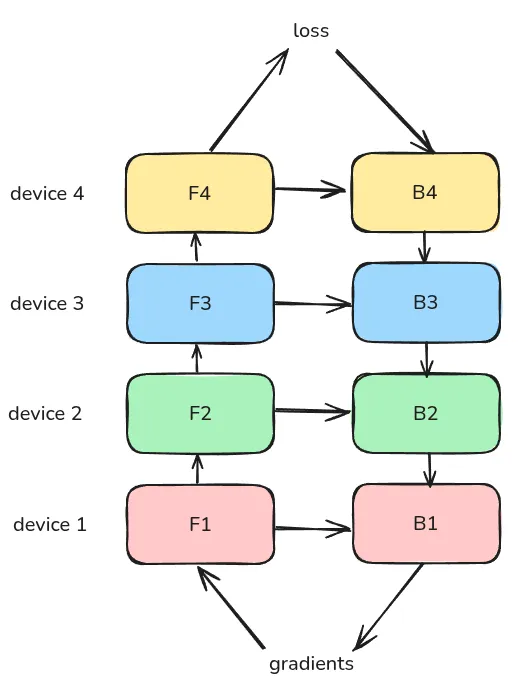
上面的方法称为 naive PP.
示意图如下所示:
通信流程如下图所示
从通信流程可以看出 naive PP 存在如下问题:
- GPU 使用率低: 一个 GPU 计算时,其他所有 GPU都闲置
- 计算和通信不重叠:执行 GPU 通信时,没有 GPU 执行计算任务
- 内存需求高: 每个 GPU 都存储了对应 batch 的所有 activation.
GPipe
为了解决 naive PP 计算效率低的问题,Google 提出了 GPipe (Huang et al., 2019) GPipe (Huang et al., 2019) 的核心思想为
将一个大的 batch 拆分为若干个较小的 batch 来提高 GPU 的利用率。
这里我们假设 PP rank 为 4,我们采用与 GPipe 一致的标记,现在每个 PP rank 上都有一层或若干层 layer, 因此我们不再对其进行标注。
GPipe 通过将输入分割为多个更小的 micro batch, 来降低不同 GPU 的闲置率。 我们现在用数字来表示对应的 micro batch. 那么 GPipe 的 pipeline 如下所示
1F1B
通过使用 micro batches, 我们可以降低整体的 GPU 闲置率。 但是,我们发现,第 1 个 micro batch 的 activation 存在于整个 batch 中,这是因为其 forward pass 时最早,而 backward pass 时最晚。 因此,我们可以优化 backward 的顺序,一旦某一个 batch 完成了 forward pass, 我们就立即对其进行 backward pass 并释放对应的 activation. 这就是 1F1B (1 forward pass 1 backward pass, (Harlap et al., 2018))
对应的流程图如下所示
可以看到,每一个 micro batch 一旦完成前向传播,就立即进行反向传播。 这样这个 micro batch 对应的 activation 也可以及时释放掉。 因此,相比于 GPipe, 1F1B 的 peak memory 占用更低
Interleaving PP
尽管 1F1B 通过立即进行反向传播的策略降低了 GPU 闲置率。 但是,我们想要进一步降低闲置率就只能减少 micro batch size, 而降低 micro batch size 又会导致计算资源浪费。
Interleaving PP 提出了交错部署的策略来实现等效降低 micro batch size 的目标。
在前面的介绍中,我们都是将相邻的 layer 放到一个 PP rank, interleaving PP 则认为,我们应该交错排列 layers, 两种方式如下表所示
| Method | normal PP | Interleaving PP |
|---|---|---|
| Rank1 | (1,2,3,4) | (1,3,5,7) |
| Rank2 | (5,6,7,8) | (2,4,6,8) |
Interleaving PP 对应的 pipeline 为 TODO
ZeroBubble
我们在前面中没有介绍的一点是,反向传播所需要的时间为前向传播的 2 倍
实际上,反向传播包括两部分:
- 对权重的梯度,其梯度不影响其他部分
- 对输入的梯度,其梯度影响前一层的梯度
ZeroBubble 基于上面这个事实,进一步降低了整体的 GPU 闲置率。 其核心思想在于
反向传播过程中,解耦权重梯度计算与输入梯度计算,将权重梯度计算填充到何时的位置上。
ZeroBubble 给出了两种模式
H2 对应的流程图为
DualPipe
DualPipe (DeepSeek-AI et al., 2025; Li & Hoefler, 2021) 的核心思想在于
一套 PP pipeline 中同时部署正向模型和反向模型。
| Method | normal PP | DualPipe |
|---|---|---|
| Rank1 | (1, 2) | (1,8) |
| Rank2 | (3,4) | (2,7) |
| Rank1 | (5,6) | (3,6) |
| Rank2 | (7,8) | (4,5) |
Optimization: TODO
Analysis
TODO
作者首先定义 notation 如下表所示
| notation | description |
|---|---|
| number of layers | |
| weights of a layer | |
| forward function of a layer | |
| forward of a partition | |
| backward of a partition | |
| number of partitions | |
| batch size | |
| micro batch size |
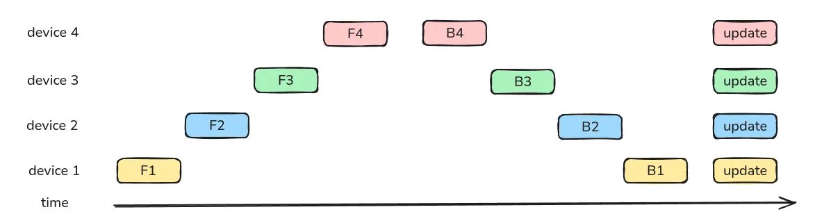
首先是 naive pipeline parallelism (naive PP), 我们的输入为一个 batch, 然后我们依次计算 , 通信传输,计算 , 计算完成之后,我们再进行反向传播,更新参数。最后继续下一个 batch 的计算。
总体的过程如下图所示
下面是一个按照时间轴给出的例子
naive PP 的问题在于,每个时刻只有一个 GPU 在工作,GPU 的利用效率很低。因此,GPipe 的做法在于将一个 batch 切分为 个更小的 micro-batch, 下面是一个 的例子
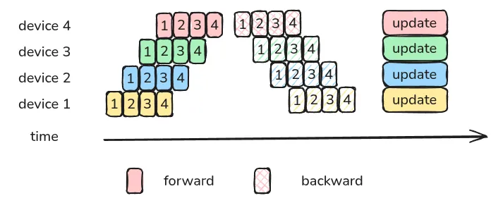
通过切分更小的 batch,我们可以提高 GPU 的利用率
接下来作者分析了 GPipe 的 bubble 情况,bubble 指的是 PP 过程中的 GPU idle time.
对于 naive PP 来说,一个 GPU 工作时,其余 GPU 都处于空闲状态,因此其 bubble 为
总的计算时间为
从而 bubble rate 为
当 时,我们有 , 也就是说,当前训练的 GPU 空闲率为 .
对于 GPipe 来说,由于我们将一个 batch 拆分为了更小的 batch, 我们可以提高 GPU 的利用率。
此时,我们的 bubble time 仍然是 . 但是,现在同一时刻工作的 GPU 变多了,从上面的示意图可以看到,前向过程所需要的时间为第一个 micro batch 运行的时间加上 个 batch 运行所需要的时间,反向同理,因此,GPipe 的总计算时间为
从而 GPipe 的 bubble rate 为
当我们令 时,我们有 , 可以看到,通过提高 micro batch 数量,我们可以显著降低 bubble rate.
对于 naive PP 来说,我们需要缓存每一层的输入,因此 activation memory 为 , 而使用 activation checkpointing 之后,我们现在的 activation memory 为
其中第一项代表了 boundary activation, 第二项代表了 Internal activation.
作者在 image classification, machine translation 任务上进行了实验。
作者还进一步分析了影响 GPipe 性能的因素,结果如下图所示
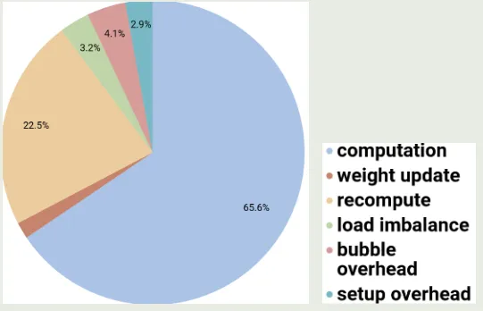
可以看到,activation checkpointing 是 GPipe 的主要开销来源。
- DeepSeek-AI, Liu, A., Feng, B., Xue, B., Wang, B., Wu, B., Lu, C., Zhao, C., Deng, C., Zhang, C., Ruan, C., Dai, D., Guo, D., Yang, D., Chen, D., Ji, D., Li, E., Lin, F., Dai, F., … Pan, Z. (2025). DeepSeek-V3 Technical Report. https://arxiv.org/abs/2412.19437
- Harlap, A., Narayanan, D., Phanishayee, A., Seshadri, V., Devanur, N., Ganger, G., & Gibbons, P. (2018). Pipedream: Fast and efficient pipeline parallel dnn training. arXiv Preprint arXiv:1806.03377.
- Huang, Y., Cheng, Y., Bapna, A., Firat, O., Chen, M. X., Chen, D., Lee, H., Ngiam, J., Le, Q. V., Wu, Y., & Chen, Z. (2019). GPipe: Efficient Training of Giant Neural Networks using Pipeline Parallelism. https://arxiv.org/abs/1811.06965 back: 1, 2
- Li, S., & Hoefler, T. (2021). Chimera: efficiently training large-scale neural networks with bidirectional pipelines. Proceedings of the International Conference for High Performance Computing, Networking, Storage and Analysis, 1–14.
Expert Parallelism
Shazeer (Shazeer et al., 2017)
EP 的计算分为以下步骤:
- router computation, 用于选取 topK 专家
- permute, 将每个专家匹配的到的 token 收集到一起方便传输
- all-to-all dispatch, 将不同专家的 token 分配给不同专家
- expert computation, 不同专家计算对应的输出
- all-to-all combine, 将不同专家的输出进行聚合
计算 pipeline 如下所示: TODO
一般来说,EP rank 和 TP rank 一致,这样可以简化计算,但是也导致EP不再是一个独立的scaling axis.
Composer 2.5 对这个进行了优化。
DeepSeek-V4 进一步实现了细粒度的 EP 优化
Analysis
Optimization
Training
Inference
DeepSeek-V4 (DeepSeek-AI, 2026)
MiniMax-01 [@MiniMax-01] 中进一步提出了 ETP, 用于将 EP 和 TP 结合起来
- DeepSeek-AI. (2026). DeepSeek-V4: Towards Highly Efficient Million-Token Context Intelligence. https://huggingface.co/deepseek-ai/DeepSeek-V4-Pro/blob/main/DeepSeek_V4.pdf
- Shazeer, N., Mirhoseini, *Azalia, Maziarz, *Krzysztof, Davis, A., Le, Q., Hinton, G., & Dean, J. (2017). Outrageously Large Neural Networks: The Sparsely-Gated Mixture-of-Experts Layer. International Conference on Learning Representations. https://openreview.net/forum?id=B1ckMDqlg
Practices
DeepSeek-V3
Acknowledgements
本文主要参考了以下内容