说明:本文参考了 nanotron/ultrascale-playbook 和 Colossal-AI Concepts
什么是分布式系统
分布式系统允许一个软件的多个组件运行在不同的机器上。与传统集中式系统不一样,分布式系统可以有效提高系统的稳健性。 一个比较比较经典的分布式就是Git,Git允许我们把代码保存在多个remote上。这样当一个remote宕机时,其他remote也能提供服务。
评估一个分布式系统的重要标准就是规模效益(scalablity),也就是说,我们希望使用8台设备应该要比4台设备快2倍。但是,由于通信带宽等原因,实际上加速比并不是和设备数量成线性关系。因此,我们需要设计分布式算法,来有效提高分布式系统的效率。
为什么需要分布式训练
我们需要分布式训练的原因主要是以下几点:
- 模型越来越大。当下(2025)领先模型如Qwen,LLaMA系列的最大模型都超过了100B [2][3]。LLaMA系列最大的模型甚至超过了1000B。Scaling law告诉我们模型表现与参数量,算力,数据量成正相关关系。
- 数据集越来越大。现在领先的模型需要的数据量基本都需要100M以上,而大语言模型训练需要的token数量也都超过了10T的量级 [2][3].
- 算力越来越强。现有最强的GPU H100其显存为80GB,拥有3.35TB/s 的带宽 (PcIe),这让训练大规模模型成为可能。
超大的模型使得我们很难在一张GPU上进行训练,甚至我们都很难使用单张GPU进行部署。而10T级的数据也也需要几个月的时间才能训练完毕。因此,如何高效利用多张GPU在大规模数据上训练超大模型就是我们需要解决的问题。
基本概念
我们先来熟悉一下分布式训练中的一些基本概念:
- Host: host (master address)是分布式训练中通信网络的主设备(main device). 一般我们需要对其进行初始化
- Node: 一个物理或虚拟的计算单元,可以是一台机器,一个容器或者一个虚拟机
- Port: port (master port)主要是用于通信的master port
- Rank: rank是通信网络中每个设备唯一的ID
- world size: world size是通信网络中设备的数量
- process group: 一个process group是通信网络中所有设备集合的一个子集。通过process group, 我们可以限制device只在group内部进行通信
我们以下图为例:
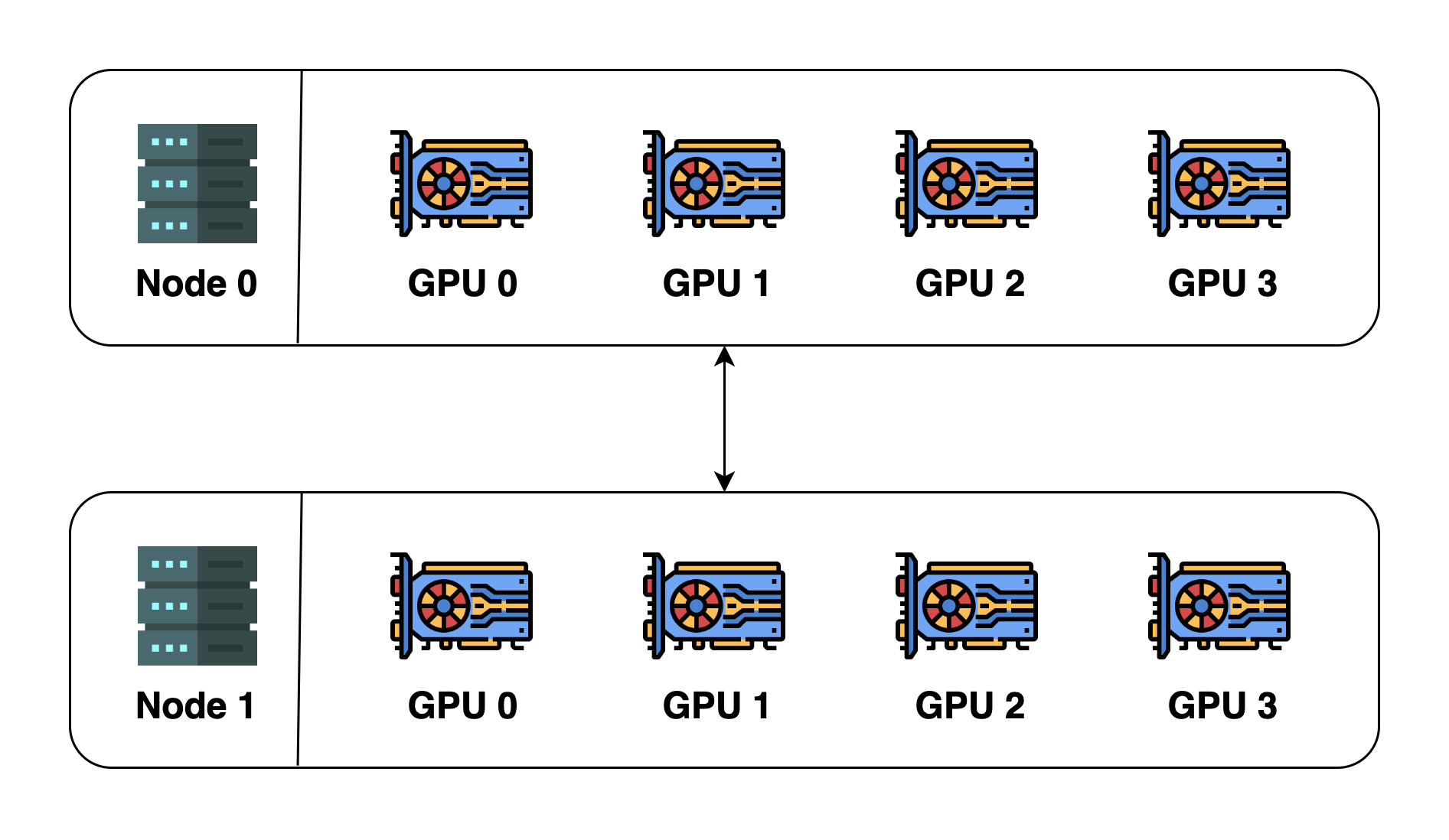 上图中一共包含2个node (2台机器),每台机器包含4个GPU (device),当我们初始化分布式环境时,我们一共启动了8个进程(每台机器4个进程),每个进程绑定一个GPU。
在初始化分布式环境之间,我们需要指定host和port。假设我们指定host为node 0和port为 29500,接下来,所有的进程都会基于这个host和port来与其他进程连接。默认的process group(包含所有device)的world size 为8. 其细节展示如下
| process ID | rank | Node index | GPU index |
|---|---|---|---|
| 0 | 0 | 0 | 0 |
| 1 | 1 | 0 | 1 |
| 2 | 2 | 0 | 2 |
| 3 | 3 | 0 | 3 |
| 4 | 4 | 1 | 0 |
| 5 | 5 | 1 | 1 |
| 6 | 6 | 1 | 2 |
| 7 | 7 | 1 | 3 |
我们可以创建一个新的process group,使其仅包含ID为偶数的process:
| process ID | rank | Node index | GPU index |
|---|---|---|---|
| 0 | 0 | 0 | 0 |
| 2 | 1 | 0 | 2 |
| 4 | 2 | 1 | 0 |
| 6 | 3 | 1 | 2 |
Remark: 注意,rank与process group相关,一个process在不同的process group里可能会有不同的rank.
通信方式
接下来,我们需要介绍一下设备间的通信方式,这是我们后面分布式训练算法的基础。根据设备数量的不同,我们可以将设备间通信分为:
- one-to-one: 两个device之间互相进行通信
- one-to-many: 一个device与多个device进行通信
- many-to-one: 多个device与一个device之间进行通信
- many-to-many: 多个device之间互相进行通信
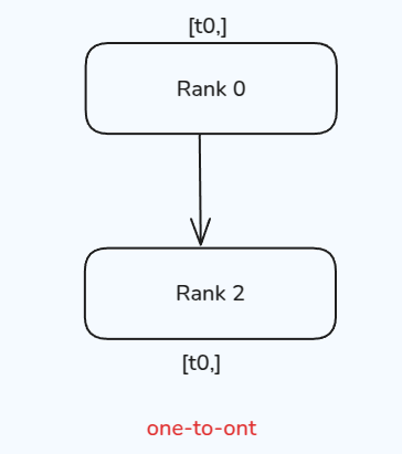
One-to-one
One-to-one的情况很简单,一个process与另一个process进行通信,通信通过 send 和 recv 完成。还有对应的 immediate版本,即 isend 和 irecv,示意图如下所示
测试代码如下:
| |
结果输出
| |
注:为了方便,后续代码仅定义函数和运行方式,
init_process()和import部分省略
send/recv的特点是在完成通信之前,两个process是锁住的。与之相反,isend/irecv 则不会加锁,代码会继续执行然后返回Work对象,为了让通信顺利进行,我们可以在返回之前加入wait()
| |
结果输出
| |
由于isend/irecv这种不锁的特性,我们不应该
- 在
dist.isend()之前修改发送的内容tensor - 在
dist.irecv()之后读取接受的内容tensor
req.wait() 可以保证这次通信顺利完成,因此我们可以在req.wait()之后再进行修改和读取。
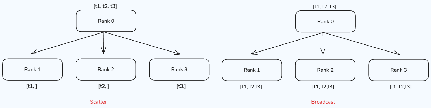
One-to-many
One-to-many 情形下,可以分为两种:scatter 和 broadcast
scatter的作用是将一个process的数据均分并散布到其他process。broadcast的作用是将一个process的数据广播到其他process。两者不同的地方在于其他process获取到的是全量数据(copy)还是部分数据(slice),其示意图如下所示
scatter 测试代码:
| |
结果输出以下内容(输出内容有优化,后续不再说明):
| |
broadcast 测试代码:
| |
结果输出:
| |
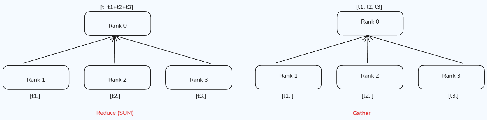
Many-to-one
Many-to-one 情形下,也可以分为两种:gather 和 reduce, Gather对应one-to-many的scatter操作,负责将多个process的内容汇聚到一起,形成一个完整的向量。而reduce的操作则是通过一个函数 $f(\cdot)$ 来把数据进行汇总,常见的函数有求和以及求平均,示意图如下所示
gather 测试代码:
| |
结果输出:
| |
reduce 测试代码:
| |
这里我们使用求和dist.ReduceOp.SUM作为我们的汇总操作,Pytorch还支持其他的reduce operations. 结果输出以下内容:
| |
Many-to-many
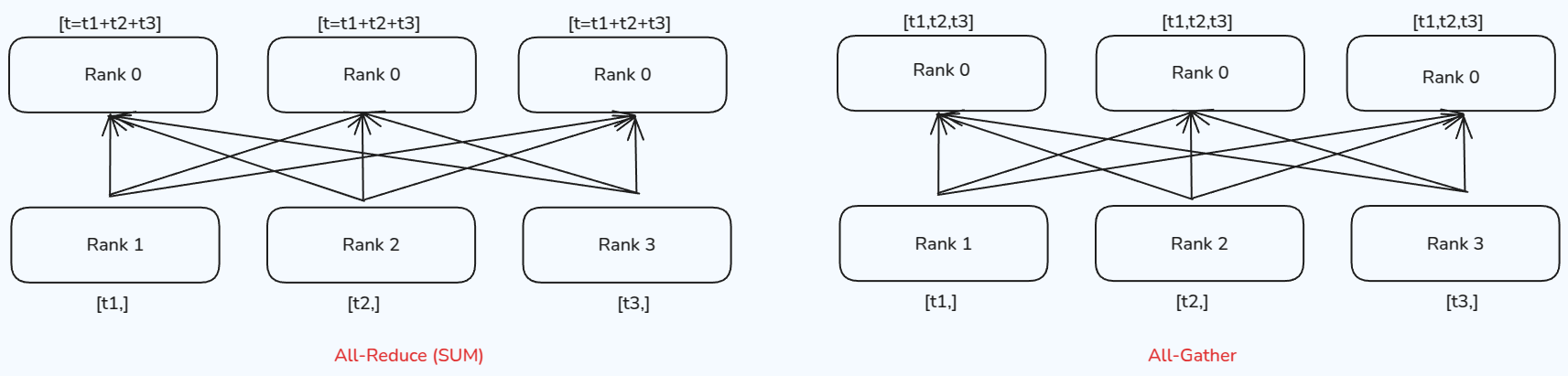
Many-to-many 情形下的两种通信方式为:All-Reduce 和 All-Gather,分别是reduce和gather的升级版,all-reduce对所有process都执行一次reduce操作,而all-gather则对所有process执行一次gather操作,其示意图如下所示
all-gather 测试代码:
| |
测试输出结果:
| |
all-reduce 测试代码:
| |
测试输出结果
| |
Barrier
除了之前这些传输数据的方式之外,我们还有Barrier,用于在所有process之间进行同步。Barrier会确保所有的process在同一时间点完成某些操作。其流程为,先让每个process完成各自的任务,然后当process到达barrier时,process会通知系统自己已到达。最后当所有process都到达barrier之后,阻塞会解除,所有process继续执行下一步操作。
barrier 测试代码
| |
结果输出
| |
可以看到,四个process的到达时间都在3s左右,这是因为rank 3需要3s才能完成当前任务
Advanced
除了前面的通信方式之外,还有 Reduce-Scatter和Ring All-Reduce,这两个通信方式等我们学习ZeRO的时候再一并讲解。