Introduction

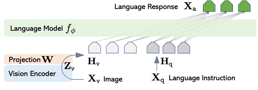
A multimodal large language model (MLLM) usually consists of three parts: an encoder $E$ that ingests the information from different modality, a large language model (LLM) that is corresponds to complete various of downstream tasks given multimodal input such as image and text, and an adaption layer $C$ that aligns features of different modality to word embedding space of the LLM. Below is an example MLLM adopting aforementioned architecture: LLaVA [1]

Efforts have been made to improve the performance of MLLMs. In this post, we aim to review the design of adaption layer and its potential effect on the downstream tasks.

Method

Suppose the hidden size of the LLM is $d$, the feature produced by encoder $E$ is $V\in\mathbb{R}^{P\times d_v}$, where $P$ is the number of features (number of visual patches if $E$ is an visual encoder) and $d_v$ is the channel dimension. The adaption layer $C$ then aligns the feature $V$ with the word embedding space with $x=C(V)\in\mathbb{R}^{Q\times d}$, where $Q$ is the number of tokens. As we can see, $C$ is actually a mapping from $\mathbb{R}^{P\times d_v}$ to $\mathbb{R}^{Q\times d}$.

Based on relationship between $d_v$ and $d$, we can divide projection layers into two types:

1. Feature-preserving adaption layer, where $P=Q$
2. Feature-compressing adaption layer, where $P>Q$.

Feature-preserving adaption layer

Feature-preserving adaption layer does not change the number of features extracted by $E$. It is used by LLaVA [1] and LLaVA 1.5 [2]. In LLaVA, the adaption layer is a linear layer [2], which is given by $x = VW^T, \text{ where } W\in\mathbb{R}^{d\times d_v}$ the code reads as:

# linear layer
adaption_layer = nn.Linear(config.hidden_size, config.num_features)

In LLaVA 1.5 , the adaption layer is a two-layer MLP, which is adopted be various of following works. It is given by $x = \phi(VW_1^T)W_2^T$ where $W_1\in\mathbb{R}^{d\times d_v}$, $W_2\in\mathbb{R}^{d\times d}$, $\phi$ is a activation function, specified as nn.GELU(). The code reads as:

# two-layer MLP
adaption_layer = nn.Sequential(
    nn.Linear(config.num_features, config.hidden_size),
    nn.GELU(),
    nn.Linear(config.hidden_size, config.hidden_size)
)

Feature-compressing adaption layer

The feature compression adaption layers can be categorized into three types:

1. average pooling
2. attention pooling
3. convolution mapping

They usually comprise two steps:

1. reduce the number of features from $P$ to $Q$ with a pooling operation: $f' = \mathcal{P}(f)\in\mathbb{R}^{Q\times d_v}$
2. project compressed features $f'$ to word embedding space with a transformation $\mathcal{T}$: $x = \mathcal{T}(f')\in\mathbb{R}^{Q\times d}$

Average pooling This type of adaption layers use an average pooling as $\mathcal{P}$ to reduce the number of tokens, followed by a two-layer MLP as $\mathcal{T}$, which is the same as LLaVA 1.5: $f'_i = \frac{1}{n}\sum_{j=1}^{n}f_{(i-1)n+j}, i=1,\dots,Q$

Perceiver Resampler This type of adaption layers use an cross-attention layer as $\mathcal{P}$, the transformation $\mathcal{T}$ is also the same as LLaVA 1.5. $K = W_kf\in\mathbb{R}^{d_c}, V=W_vf\in\mathbb{R}^{d_c}, f'=\mathrm{softmax}\left(\frac{QK^T}{\sqrt{d_c}}\right)V\in\mathbb{R}^{Q\times d_v}$ where $W_k, W_v\in\mathbb{R}^{d_c\times d_v}$ and $Q\in\mathbb{R}^{Q\times d_c}$ is a learnable query.

class PerceiverResampler(nn.Module):
    def __init__(self, num_queries, hidden_size, num_features, num_heads):
        self.num_queries = num_queries
        self.hidden_size = hidden_size
        self.num_features = num_features

        self.query_tokens = nn.Parameter(torch.zeros(self.num_queries, self.num_features), requires_grad=True)
        self.query_tokens.data.normal_(mean=0.0, std=0.02)

        self.attention = nn.MultiheadAttention(hidden_size, num_heads)
        self.layer_norm_kv = nn.LayerNorm(hidden_size)
        self.layer_norm_q = nn.LayerNorm(hidden_size)

    def forward(self, x, attention_mask=None):
        x = self.layer_norm_kv(x)
        x = x.permute(1, 0, 2)

        N = x.shape[1]
        q = self.layer_norm_q(self.query_tokens)
        q = q.unsqueeze(1).repeat(1, N, 1)
        out = self.attention(q, k, v, attention_mask=attention_mask)[0]

        out = out.permute(1, 0, 2)

adaption_layer = nn.Sequential(
    PerceiverResampler(num_queries, hidden_size, num_features, num_heads),
    MLP(hidden_size, intermediate_size, hidden_size)
)

C-Abstractor This type of adaption layers use a combination of convolution layer and averaging pooling as $\mathcal{P}$. $\mathcal{T}$ is defined as an additional convolution layers. $f_i' = \frac{1}{n}\sum_{j=1}^n w_jf_{(i-1)n+j},\quad x_i = \sum_{k=-K}^Kw_k'f_{i+k}'$ where $W=[w_1,\dots,w_n]^T\in\mathbb{R}^n$ and $W'=[w_1,\dots,w_n]^T\in\mathbb{R}^{2K}$ are the weights of the convolution layers.

D-Abstractor aa

Usages

Comparisons

1. LLaVA
2. LLaVA 1.5
3. LLaVA adaption layer code
4. survey