本文中，我们将介绍如何计算 LLM 在训练和推理过程中的内存需求以及简要介绍对应的优化方法。

Introduction

我们在本文中回答的核心问题为：

在训练和推理时 LLM 所需要的内存是多少？如何进行优化内存占用？

为了回答这两个问题，我们需要回答以下问题：

1. 训练和推理时的内存由哪几部分组成？
2. 训练和推理过程中哪个阶段是 memory-bound? 哪个阶段是 compute bound?
3. 训练和推理过程中如何进行优化？

我们将首先介绍如何计算 LLM 在训练阶段和推理阶段的内存。接下来，我们针对可优化部分进行分析以及介绍相应的优化算法。后续，我们将针对每部分的优化进行详细介绍

Background

首先我们介绍一下使用的 notation, 这与之前参数量，FLOPs 计算使用的 notation 基本一致。需要注意的是，我们直接使用参数量 $P$ 这个记号，这部分在 LLM parameter analysis 中已经进行了详细介绍，因此我们略过这部分。

Assumption

1. 没有特别说明的话，我们使用 BF16/FP16 作为精度，此时每个参数需要 $2$ byte 来表示
2. 不使用 dropout (现代大模型普遍没有 dropout)

Computation

Overview

我们首先给出训练和推理阶段各部分的内存需求，然后我们给出详细的计算公式

Training

LLM 训练阶段对的内存开销包含三部分

Weights

我们在前面已经介绍了如何计算大语言模型的参数量，这里我们就直接记为 $P$, 由于我们使用单精度，因此所需要的内存为 $2P$.

Activation

激活值（activation）是前向传播过程中产生的中间张量，反向传播计算梯度时需复用这些张量，因此训练阶段需全程存储。我们用一个简单的例子来进行说明，假设我们有一层神经网络，定义为

那么在反向传播过程中，我们有

也就是说，在计算第 $l$ 层的参数对应的梯度时，我们需要知道对应的输入 $\mathbf{a}_{l-1}$.

接下来，我们通过计算图来分析 LLM 所需要的 activation

Attention Attention 的计算图如下所示 （见 attention-computation-graph）

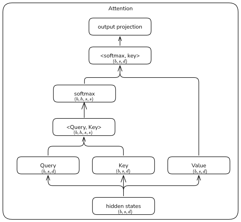
根据计算图，对应的 activation 为（注：这里我们不做任何优化，仅此理论上进行分析）：

1. query, key, value projection: 共享输入，对应的 activation 大小为 $2bsd$.
2. $Q^TK$ : $Q$, $K$ 都需要保存，大小为 $4bsd$.
3. softmax: 需要保存 $2bhs^2$ 大小的输入
4. weighted sum of values: 两者都需要保存，前者大小为 $2bhs^2$, 后者大小为 $2bsd$
5. output projection layer: 需要保存输入，大小为 $2bsd$.

因此 attention 部分总共需要 $\boxed{10sbd+4bhs^2}$.

FFN FFN 计算图如下所示（见 FFN-computation-graph）

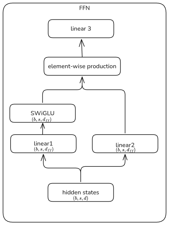
根据计算图，对应的 activation （我们假设 MLP 是一个基于 SwiGLU 的 dense MLP, 其 hidden size $d_{ff}=8/3d$,）：

1. MLP 的第一层输入大小为 $2sbd$,
2. MLP 的第二层输入大小为 $16/3sbd$,
3. SwiGLU 的输入为 $16/3sbd$

因此总的 activation 大小为 $\boxed{18sbd}$.

LayerNorm LayerNorm 需要保存输入，大小为 $\boxed{2bsd}$.

以上三部分相加，我们就得到单一 transformer layer 所需要的 activation:

output output 部分的计算图如下所示

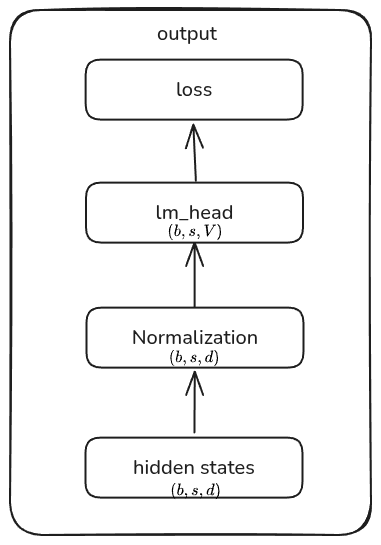
根据计算图，对应的 activation 为：

1. normalization 的输入大小为大小为 $2sbd$
2. lm_head 的输入大小为 $2sbd$
3. loss 的输入大小为 $2bsV$

从而输出部分的 activation 大小为

因此，总的 activation 为

Gradients & Optimizer States

现代优化器一般会使用高阶近似以及混合精度训练来提高训练的效率，这部分高阶近似也需要考虑内存占用。

Gradients 当 gradient 和 weight 精度一致时，对应的内存消耗一致，为 $\boxed{2P}$.

Optimizer states AdamW 优化器会保存一阶和二阶动量，以及一份 master weights, 精度一般为 FP32:

1. FP32 master weights: $4P$
2. FP32 first-order momentum: $4P$
3. FP32 second-order momentum: $4P$

因此优化器状态需要 $\boxed{12P}$ 内存。

对于其他优化器，我们也可以算出对应的内存需求，下表总结了 AdamW, bitsandbytes 和 SGD 三种 optimizer

最终，训练阶段所需要的内存为

下面我们展示 LLaMA 系列训练时不同部分的内存占比 (batch size=64, AdamW, GB)

Inference

LLM 推理阶段对的开销包含三部分

weight memory 的内存占用为 $\boxed{2P}$. activation 内存占用比较小，transformer-math 给出了一个经验值，即

该经验值适用于 batch size = 1 的自回归推理场景。weight 和 activation 这两部分开销只与模型本身有关，第三部分 KV cache 则与我们的生成内容长度相关，下面我们详细进行介绍

Key Value Cache

Key Value Cache (KV Cache) 是 LLM 在推理过程中为了避免重复计算历史 token 对应的 key 和 value 而使用的一个空间换时间的缓存机制。

在 LLM 推理阶段，我们是 token-by-token 进行生成的，每次 attention 的计算都有如下形式

这里 $\mathbf{q_t}$ 是当前 token $\mathbf{x}_t$ 对应的 query, $\mathbf{k}_{:,t}$ 和 $\mathbf{v}_{:,t}$ 是历史 token $[\mathbf{x_1},\dots,\mathbf{x_t}]$ 对应的 key 和 value. 当我们处理下一个 token $\mathbf{x}_{t+1}$ 时， 对应的计算变成了

也就是说，我们每生成一个 token, 都要重新计算一次历史 token 对应的 key 和 value, 因此生成一个包含 $s$ 个 token 的 sequence 时，每个 token 都需要计算其前序 token 的 key 和 value, 其对应的计算量为

因此，一个自然的想法就是缓存历史 token 对应的 key 和 value, 在生成新的 token 时，我们只需从内存中加载计算好的结果，然后计算当前 token 对应的值 $W_K\mathbf{x}_{t+1}$ 和 $W_V\mathbf{x}_{t+1}$ 即可，这就是 KV cache. 使用 KV cache 之后，我们每次生成新的 token 时，仅需要计算当前 token 对应的 key 和 value, 此时总的计算复杂度为 $\mathcal{O}(s)$, 对应的空间复杂度为 $\mathcal{O}(s)$. 也就是以空间换时间。

容易推导出一个基于 Multi-head attention LLM 的 KV cache 如下

可以看到，KV Cache 占用不仅与模型配置有关，还与生成的 sequence length 有关，生成的 token 越多，KV Cache 这部分占用越高。

具体细节见 KV cache

最终，推理阶段模型本身的内存占用为

我们还是以 LLaMA 系列为例，结果如下 (batch size=1, GB, 括号里为 sequence length)

可以看到，随着输出长度增加，KV cache 的开销占比也逐渐了超过模型权重的内存占用。而实际中 KV cache 往往因 page granularity、padding 和 fragmentation 略高于理论值。

Summary

我们将上面的结果汇总起来就得到下表的结果。

Analysis & Optimizations

接下来，我们将简单介绍一下如何优化训练和推理过程中的内存占用，我们将优化方法总结如下表所示。后面我们将一一进行详细介绍

Training

Mixed Precision Training

混合精度训练的核心思想是计算量大的模块使用低精度，计算量小的模块使用高精度。细节见 Mixed precision training, 最近的 DeepSeek-V3 还进一步使用了 FP8 精度进行训练，大幅度提高了训练效率。

Data Parallelism

第一个并行策略是数据并行 (data parallelism), 其基本思想是把模型复制到多个 GPU 上，并行处理数据，然后对 loss 进行求和再进行反向传播。现在最常使用的是微软提出的 ZeRO, 其核心思想为把 optimizer states, gradients, weights 分布到不同的 GPU 上，然后需要的时候再汇总到一起。ZeRO 根据切分的部分不同可以分为三种策略，如下图所示

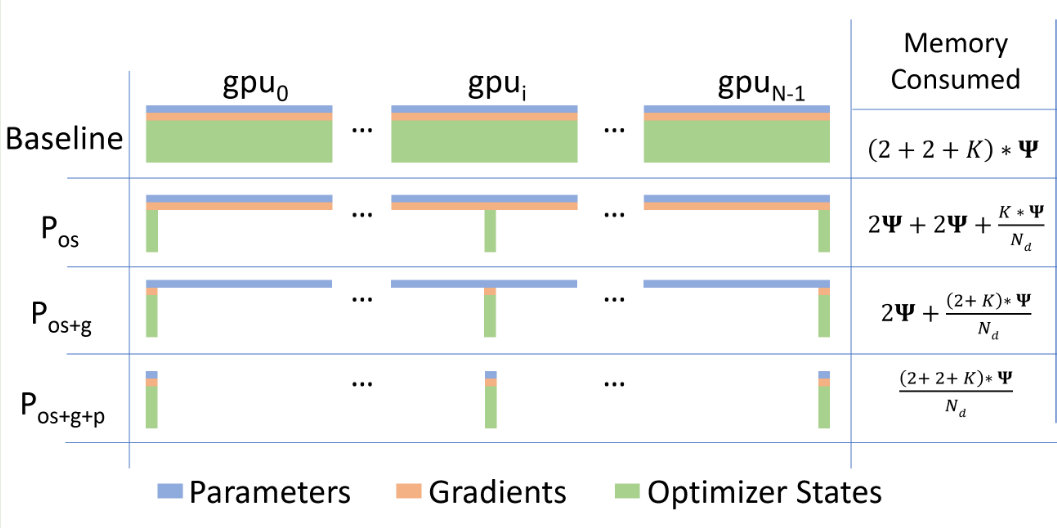
如上图所示，在 baseline 场景下，我们每个 GPU 上都保存有一份模型的 optimizer states, gradients, weights, 这就限制了 batch size, 进而降低了整体的计算效率。

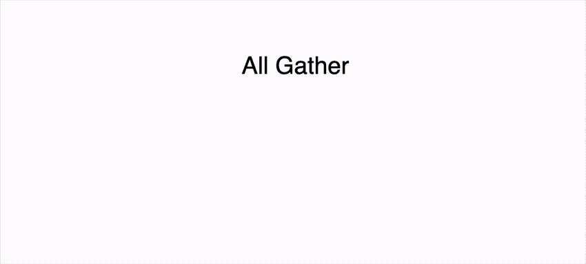
ZeRO 的关键改进在于利用 GPU 可以互相通信的性质来将 tensor 存储在不同的 GPU 上，这时每个 GPU 上不再保存完整的复制，而是独特的一部分数据，在参与计算时，GPU 通过 all gather 来把数据汇总在一起，如下图所示

ZeRO1 只对 optimizer states 进行 shard, 因此其内存占用为

ZeRO2 在 ZeRO1 的基础上进一步对 gradient 也进行 shard, 其内存占用为

ZeRO3 在 ZeRO2 的基础上对 weight 也进行 shard, 其内存占用为

一般来说，我们比较少使用 ZeRO3, 因为其通信开销变为了原来的 1.5 倍。细节介绍见 ZeRO

Activation Checkpointing

上一节我们介绍了使用 DP 来减少固定部分 (weight, optimizer states, gradients) 部分的占用，但实际上训练时占用部分更多的是 activation, 这部分内存占用会严重影响 batch size 的设置进而影响整体计算效率。我们对固定部分（与模型参数量相关）和非固定部分（与 batch size 相关）进行一个对比，结果如下所示

我们可以看到，虽然训练时 batch size 越大越好，但是由于 activation 也会随之增大，batch size 可能只能使用一个非常小的值。下图是 LLaMA 系列在 $b=64$ 时不同部分的内存占用：

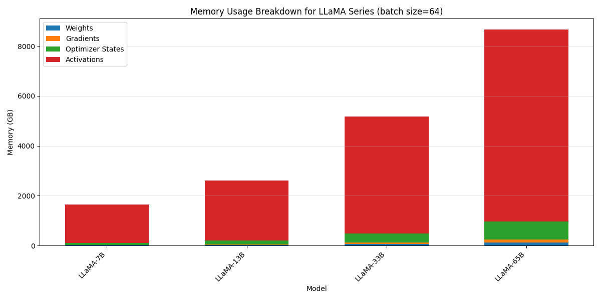
从图表可看出，LLaMA-65B 在 batch size=64 时，激活值占用内存超 80%，远高于权重 / 梯度 / 优化器状态，而且随着 batch size 增加，这个比例会进一步上升。

为了解决这个问题，我们一般会使用 activation checkpointing 方法，这个方法是一个通过重新计算中间激活值，来减少内存占用的方法。其核心思想在于用计算复杂度换空间复杂度。Reducing Activation Recomputation in Large Transformer Models 给出了不同的 checkpointing 策略，需要的算力也不同相同，我们下表进行总结

一般来说我们会结合 model parallelism 和 selective checkpointing 来实现一个均衡

Model Parallelism

与 DP 在数据维度上进行切分不同，model parallelism 通过对模型进行切分来提高内存使用效率。Model Parallelism 又可以分为 Pipeline Parallelism (PP) 和 Tensor Parallelisim (TP)

通过 PP 和 TP 我们可以将模型切分部署在多个 GPU 上进而减少内存占用，对应的计算方式为

实际情况中，我们还可以结合 ZeRO 以及 Model Paralelism, 我们根据 PP degree 和 TP degree 来决定 DP degree

最终，我们把以上优化技巧汇总起来就得到 (假设我们采用 ZeRO1 和 Model Parallelism)

这里> activation 中 被 tensor-parallel 的部分 按 TP degree 缩减。

关于 Parallelism 的具体细节见 Parallelism tutorial

Flash Attention

在前面的分析中，我们给出了 attention softmax 这一部分的 activation 为 $2bhs^2$ 而 flashattention 通过 tiling 和 online-softmax 降低了这一部分的内存占用，进而提高整体的效率。

具体细节见 flash attention

Inference

Quantization

quantization 是用低精度加载模型权重从而降低推理阶段模型参数内存占用的一个方法。比如说原始模型使用了 BF16 精度，那么我们可以通过使用 int8 量化来将模型权重对应的内存从 $2P$ 降低到 $P$. 现在一些模型还会在训练阶段就加入 quantization, 比如 quantization aware training 以及 post-training quantization 等。这部分细节可以参考 Efficient Large Language Models: A Survey

KV Cache Optimization

我们在前面已经介绍了 KV cache 可以通过以空间换时间来提高计算效率，但是随着输出长度增加，对应的 KV cache 也会越来越大，因此目前有相当一部分工作旨在降低 KV cache 占用，比如 KV Cache compression, quantization 等。这部分细节可以参考 A Survey on Large Language Model Acceleration based on KV Cache Management

Attention

实际上，相当一部分工作都是通过优化 attention 来降低

见 attention tutorial

Inference Framework

现在也有一些推理框架专注于提高 LLM 的推理效率，下面是两个比较流行的推理框架

• SGLang: 定制化强，适用于复杂任务如 RL 推理等
• vLLM: 简单高效

对应的轻量化推理框架为

• nano-vLLM
• mini-SGLang

这部分

Conclusion

在本文中，我们详细介绍了 LLM 在训练和推理阶段的内存占用开销以及简要介绍了对应的优化方法。关键结论为：

• 训练阶段内存核心瓶颈是激活值（随 batch size / 序列长度线性增长），推理阶段核心瓶颈是 KV Cache（随序列长度增长）；
• 训练优化优先通过 ZeRO（多卡）+ activation checkpointing（单卡）降低内存，推理优化优先通过 KV Cache 优化 + 量化降低内存；
• 所有内存计算均为理论值，实际落地需考虑显存碎片、硬件特性、通信开销等工程因素。

需要注意的是，所有内存计算均为理论值，实际落地需考虑显存碎片、硬件特性、通信开销等工程因素。下一步，我们将分别针对不同的优化方法来进行展开并详细介绍。

References

• transformer-math
• transformer inference arithmetic
• https://zhuanlan.zhihu.com/p/687226668
• Reducing Activation Recomputation in Large Transformer Models
• https://blog.eleuther.ai/transformer-math/
• A Survey on Large Language Model Acceleration based on KV Cache Management
• Efficient Large Language Models: A Survey

Appendix

Activation Visualization

LLaMA 系列的配置如下表所示

对应的可视化代码如下

 1
 2
 3
 4
 5
 6
 7
 8
 9
10
11
12
13
14
15
16
17
18
19
20
21
22
23
24
25
26
27
28
29
30
31
32
33
34
35
36
37
38
39
40
41
42
43
44
45
46
47
48
49
50
51
52

import numpy as np
import matplotlib.pyplot as plt

def compute_memory(L, d, h, h_d, V, s, P, b):
    weights = 2 * P
    gradients = 2 * P
    optimizer_states = 12 * P
    activations = L*s*b*(32 * d + 4 * h * s) + (4 * b * s * d + 2 * b * s * V)
    return {
        "weights": weights,
        "gradients": gradients,
        "optimizer_states": optimizer_states,
        "activations": activations,
    }


b = 64  # batch size for memory calculation
memory_data = {}

for model, params in models.items():
    memory = compute_memory(params["L"], params["d"], params["h"], params["h_d"], params["V"], params["s"], params["P"], b)
    memory_data[model] = memory

fig, ax = plt.subplots(figsize=(12, 6))

model_names = list(memory_data.keys())
GB = 1024 ** 3  # 1 GB in bytes

weights = [memory_data[m]["weights"] / GB for m in model_names]
gradients = [memory_data[m]["gradients"] / GB for m in model_names]
optimizer_states = [memory_data[m]["optimizer_states"] / GB for m in model_names]
activations = [memory_data[m]["activations"] / GB for m in model_names]

x = np.arange(len(model_names))
width = 0.6

# Stacked bar chart
p1 = ax.bar(x, weights, width, label='Weights')
p2 = ax.bar(x, gradients, width, bottom=weights, label='Gradients')
p3 = ax.bar(x, optimizer_states, width, bottom=np.array(weights) + np.array(gradients), label='Optimizer States')
p4 = ax.bar(x, activations, width, bottom=np.array(weights) + np.array(gradients) + np.array(optimizer_states), label='Activations')

ax.set_xlabel('Model')
ax.set_ylabel('Memory (GB)')
ax.set_title(f'Memory Usage Breakdown for LLaMA Series (batch size={b})')
ax.set_xticks(x)
ax.set_xticklabels(model_names, rotation=45, ha='right')
ax.legend()
ax.grid(axis='y', alpha=0.3)

plt.tight_layout()
plt.show()