Introduction
随着模型参数变大,现有的 GPU 已经很难使用单一 GPU 来训练模型。对于多 GPU 训练场景,目前主要采用了 pipeline parallelism, 比如 GPipe 等,但是,这些策略需要我们对代码进行比较大的改动,这提高了开发成本。
为了解决多 GPU 训练大规模 LLM 的效率,降低开发成本,目前主要使用了 model parallelism 策略,即对模型进行切分部署在多个 GPU 上。model parallelism 有两种范式:
- pipeline parallelism (PP): 将模型按照 layer 进行切分,如 GPipe 等,这种方法的问题是需要额外的逻辑来处理通信以及存在 pipeline bubbles
- tensor parallelism (TP): 将模型的按照权重进行切分,部署在不同的 GPU 上。
作者在本文中基于 TP 策略来对 attention, FFN layer 进行简单改动来实现训练效率的提升。
作者通过实现验证了 tensor parallelism 的有效性和高效率,结果发现在 512 张 GPU 的场景下,TP 可以达到 $76\%$ 的 scaling efficiency (相比于 1 张 GPU 带来的性能提升)
Method
作者使用的 transformer 架构如下图所示
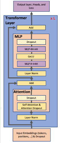
本文中,作者探究了 BERT 和 GPT-2 两种架构。
首先,我们假设 transformer layer 输入为 $X\in\mathbb{R}^{bs\times d}$, 这里 $b, s$ 分别为 batch size, sequence length, 接下来我们介绍如何针对 FFN, attention 以及 embedding 构建 TP 策略
FFN
论文中使用的 FFN 为 Linear-GeLU-Linear 的结构,对应第一层权重为 $W_1\in\mathbb{R}^{d\times d_{ff}}$, 第二层权重为 $W_2\in\mathbb{R}^{d_{ff}\times d}$, 对应数学表达式为
$$
Y = \mathrm{GeLU}(XW_1)W_2\in\mathbb{R}^{bs\times d}
$$我们首先对 $W_1$ 按照 column 进行切分,得到
$$
W_1 = [W_{11}, W_{12}]\in\mathbb{R}^{d\times d_{ff}}, \text{ where } W_{11}\in\mathbb{R}^{d\times d_1}, W_{12}\in\mathbb{R}^{d\times d_2}, d_1+d_2=d_{ff}
$$这里 $d_1, d_2$ 与我们并行的 GPU 数 (x-way TP) 相关,这样,我们就有
$$
\mathrm{GeLU}(XW_1) = \mathrm{GeLU}(X[W_{11}, W_{12}]) = \mathrm{GeLU}([XW_{11}, XW_{22}]) = [\mathrm{GeLU}(XW_{11}), \mathrm{GeLU}(XW_{12})]
$$从而我们可以分别将 $W_{11}$ 和 $W_{12}$ 部署在两个 GPU 上,然后并行计算。
论文中还介绍如果我们对 $W_1$ 按照 row 进行切分,则最终由于 $\mathrm{GeLU}(A+B)\neq \mathrm{GeLU}(A)+\mathrm{GeLU}(B)$ 计算时会产生一次额外的同步。
接下来,对于 $W_2$, 我们按照 row 进行切分得到
$$
W_2 = \begin{bmatrix}
W_{21}\\
W_{22}
\end{bmatrix}\in\mathbb{R}^{d_{ff}\times d}, \text{ where }W_{21}\in\mathbb{R}^{d_1\times d}, W_{22}\in\mathbb{R}^{d_2\times d}, d_1+d_2=d_{ff}
$$计算时,我们有
$$
\mathrm{GeLU}(XW_1)W_2 = [\mathrm{GeLU}(XW_{11}), \mathrm{GeLU}(XW_{12})]\begin{bmatrix}
W_{21}\\
W_{22}
\end{bmatrix} = \mathrm{GeLU}(XW_{11})W_{21} + \mathrm{GeLU}(XW_{12})W_{22}
$$可以看到,通过按照 row 进行切分,我们可以将 $W_{11}, W_{21}$ 部署在一个 GPU 上,将 $W_{12}, W_{22}$ 部署在另一个 GPU 上,分别计算出 $\mathrm{GeLU}(XW_{11})W_{21}$ 和 $\mathrm{GeLU}(XW_{12})W_{22}$ 之后,再通过一此 all-reduce 操作得到最终的输出结果。计算图如下所示
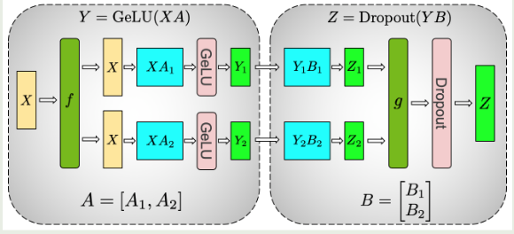
这里 $f$ 和 $g$ 是两个对偶算子,代表了 TP 产生的额外通信开销
| operator | forward | backward |
|---|
| $f$ | identity | all-reduce |
| $g$ | all-reduce | identity |
如果说我们使用的是 SwiGLU FFN, 即
$$
Y = (XW_3\odot \mathrm{Swish}(XW_1))W_2
$$我们按照 column 对 $W_1, W_3$ 进行切分,按照 row 对 $W_2$ 进行切分(假设我们有 2 个 GPU),得到
$$
\begin{aligned}
W_1 &= [W_{11}, W_{12}]\in\mathbb{R}^{d\times d_{ff}}, \text{ where } W_{11}\in\mathbb{R}^{d\times d_1}, W_{12}\in\mathbb{R}^{d\times d_2}, d_1+d_2=d_{ff}\\
W_3 &= [W_{31}, W_{32}]\in\mathbb{R}^{d\times d_{ff}}, \text{ where } W_{31}\in\mathbb{R}^{d\times d_1}, W_{32}\in\mathbb{R}^{d\times d_2}, d_1+d_2=d_{ff}\\
W_2 &= \begin{bmatrix}
W_{21}\\
W_{22}
\end{bmatrix}\in\mathbb{R}^{d_{ff}\times d}, \text{ where }W_{21}\in\mathbb{R}^{d_1\times d}, W_{22}\in\mathbb{R}^{d_2\times d}, d_1+d_2=d_{ff}
\end{aligned}
$$然后我们将 $W_{11}, W_{31}, W_{21}$ 放在第一个 GPU 上,将 $W_{12}, W_{32}, W_{22}$ 放在第二个 GPU 上,此时,
$$
\begin{aligned}
\mathrm{Swish}(XW_1) &= \mathrm{Swish}(X[W_{11}, W_{12}])
= \mathrm{Swish}([XW_{11}, XW_{12}])=[\mathrm{Swish}(XW_{11}, \mathrm{Swish}(XW_{12}]\\
XW_3\odot \mathrm{Swish}(XW_1) &= [XW_{31}, XW_{32}]\mathrm{Swish}(XW_1) = [XW_{31}\mathrm{Swish}(XW_{11}), XW_{32}\mathrm{Swish}(XW_{12})]\\
Y = (XW_3\odot \mathrm{Swish}(XW_1))W_2&=(XW_3\odot \mathrm{Swish}(XW_1))\begin{bmatrix}
W_{21}\\
W_{22}
\end{bmatrix} = XW_{31}\mathrm{Swish}(XW_{11})W_{21}+ XW_{32}\mathrm{Swish}(XW_{12})W_{22}
\end{aligned}
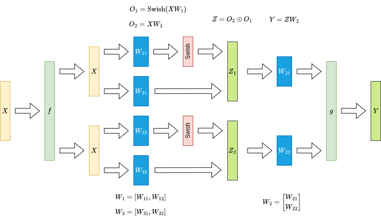
$$这样我们通过一次 all-reduce 也可以完成 SwiGLU FFN 的 tensor parallelism, 示意图如下所示
Attention
Attention 的处理与 MLP 非常相似,论文中的做法就是将不同 head 部署到不同 gpu 上分别进行计算,最后在计算 output projection 时再通过一次 all-reduce 来合并输出,这里我们假设有 $h$ 个 heads, 每个 head 的 dimension 为 $d_h$, 我们先对 query, key, value layer 的 weight $W_Q, W_K, W_V\in\mathbb{R}^{d\times hd_h}$ 进行切分
$$
W_Q = [W_{Q1}, \dots, W_{Qh}], W_K = [W_{K1}, \dots, W_{kh}], W_V = [W_{V1}, \dots, W_{Vh}]
$$其中 $W_{Qi}, W_{Ki}, W_{Vi}\in\mathbb{R}^{d\times d_h}$ 为每个 head 对应的 query, key, value weight. 我们将切分后的 $W_{Qi}, W_{Ki}, W_{Vi}$ 部署在一个 GPU 上(也可以将若干个 head 部署在一个 GPU 上),然后分别计算出每个 GPU 的 attention 结果,最后再进行汇总,如下所示
$$
\begin{aligned}
o_i &= \mathrm{softmax}\left(\frac{(XW_{Qi})(XW_{Ki})^T}{d_h}\right) XW_{Vi}, i=1,\dots,h\\
O &= [o_1,\dots,o_h]W_O
\end{aligned}
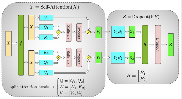
$$下面是 multi-head attention 对应的 TP 示意图
Embedding
对于 Input embedding, 作者将 embedding matrix $E\in\mathbb{E}^{V\times d}$ 按照 row 进行切分(论文中使用了转置,因此是按照 column 进行切分),得到 $E=[E_1,E_2]^T$, 这里 $E_i\in\mathbb{R}^{d\times V_i}$, $V_1+V_2=V$, 接下来我们把切分后的 embedding matrix 部署在不同的 GPU 上,由于每个 GPU 只有部分结果,因此我们还需要进行 all-reduce 来进行汇总。
而对于 output embedding, 我们也可以使用类似的做法进行切分,每个 GPU 上计算完结果之后我们还需要一个 all-gather 来汇总结果。
作者在这里还额外介绍了针对 output embedding 的优化方法,由于 embedding 的输出大小为 $[bs, V]$, 而 $V$ 通常比较大,因此,为了降低通信开销,作者将 cross-entropy-loss 与 output embedding kernel 进行融合,这样我们传输的数据量就减少到了 $bs$.
Experiments
作者首先对 GPT-2 模型进行了修正,首先将 vocab_size 从 50257 提升到 128 的倍数,即 51200. 对于 model+data parallelism, 作者固定 global batch size 为 512. (64-way DP)
配置如下表所示(head size 为 96)
| Hidden size | attention heads | layers | parameters (B) | TP | TP+DP |
|---|
| 1536 | 16 | 40 | 1.2 | 1 | 64 |
| 1920 | 20 | 54 | 2.5 | 2 | 128 |
| 2304 | 24 | 64 | 4.2 | 4 | 256 |
| 3072 | 32 | 72 | 8.3 | 8 | 512 |
对应的 scaling (使用多卡训练后,每个 GPU 相对于单卡训练的利用率)如下表所示
| parallelism | TP-1 | TP-2 | TP-4 | TP-8 | TP-1+DP-64 | TP-2+DP-64 | TP-4+DP-64 | TP-8+DP-64 |
|---|
| scaling | 100% | 95% | 82% | 77% | 96% | 83% | 79% | 74% |
Implementation
首先是 linear layer 的 TP 版本,如下所示
 1
 2
 3
 4
 5
 6
 7
 8
 9
10
11
12
13
14
15
16
17
18
19
20
21
22
23
24
25
26
27
28
29
30
31
32
33
34
35
36
37
38
39
| import torch
import torch.nn as nn
import torch.distributed as dist
class ColumnParallelLinear(nn.Module):
def __init__(self, in_features, out_features, bias=True):
super().__init__()
self.rank = dist.get_rank()
self.world_size = dist.get_world_size()
self.local_out = out_features // self.world_size
self.weight = nn.Parameter(torch.empty(in_features, self.local_out))
def forward(self, x):
out = x @ self.weight
gather_list = [torch.empty_like(out) for _ in range(self.world_size)]
dist.all_gather(gather_list, out)
return torch.cat(gather_list, dim=-1)
class RowParallelLinear(nn.Module):
def __init__(self, in_features, out_features, bias=True):
super().__init__()
self.rank = dist.get_rank()
self.world_size = dist.get_world_size()
self.local_in = in_features // self.world_size
self.weight = nn.Parameter(torch.empty(self.local_in, out_features))
def forward(self, x):
x_local = torch.chunk(x, self.world_size, dim=-1)[self.rank]
out = x_local @ self.weight
dist.all_reduce(out, op=dist.ReduceOp.SUM)
return out
|
接下来是针对 LLM 中使用的 SwiGLU FFN 进行的优化,基于前面的介绍,我们不需要对基于 column linear 进行 all-reduce, 代码如下所示
SwiGLU
 1
 2
 3
 4
 5
 6
 7
 8
 9
10
11
12
13
14
15
16
17
18
19
20
21
22
23
24
25
26
27
28
29
30
31
32
33
34
35
36
37
38
39
40
41
42
| import torch
from torch import nn
import torch.nn.functional as F
import torch.distributed as dist
world_size = 1
rank = 0
class ColumnParallelLinear(nn.Module):
def __init__(self, in_features: int, out_features: int, dtype = None):
assert out_features % world_size == 0, f"Output features must be divisible by world size (world_size={world_size})"
self.part_out_features = out_features // world_size
self.weight = nn.Parameter(torch.empty(part_out_features, part_in_features, dtype=dtype))
def forward(self, x: torch.Tensor) -> torch.Tensor:
y = x @ self.weight
return y
class RowParallelLinear(nn.Module):
def __init__(self, in_features: int, out_features: int, dtype = None):
assert in_features % world_size == 0, f"Input features must be divisible by world size (world_size={world_size})"
self.part_in_features = in_features // world_size
self.weight = nn.Parameter(torch.empty(out_features, part_in_features, dtype=dtype))
def forward(self, x: torch.Tensor) -> torch.Tensor:
y = x @ self.weight
if world_size > 1:
dist.all_reduce(y)
return y
class MLP(nn.Module):
def __init__(self, dim: int, inter_dim: int):
super().__init__()
self.w1 = ColumnParallelLinear(dim, inter_dim)
self.w2 = RowParallelLinear(inter_dim, dim)
self.w3 = ColumnParallelLinear(dim, inter_dim)
def forward(self, x: torch.Tensor) -> torch.Tensor:
return self.w2(F.silu(self.w1(x)) * self.w3(x))
|
attention
 1
 2
 3
 4
 5
 6
 7
 8
 9
10
11
12
13
14
15
16
17
18
19
20
21
22
23
24
25
26
27
28
29
30
31
32
33
34
35
36
37
38
39
40
41
42
43
44
45
46
47
48
49
50
51
52
53
54
55
56
57
| class TPMultiHeadAttention(nn.Module):
def __init__(self, d_model: int, num_heads: int, head_dim: int = None):
self.d_model = d_model
self.num_heads = num_heads
self.head_dim = head_dim if head_dim is not None else d_model // num_heads
assert self.num_heads % world_size == 0, "num_heads must be divisible by world size"
assert self.d_model == self.num_heads * self.head_dim, "d_model must equal num_heads * head_dim"
# heads of different GPU
self.local_num_heads = self.num_heads // world_size
self.local_qkv_dim = self.local_num_heads * self.head_dim
self.qkv_proj = ColumnParallelLinear(in_features=d_model, out_features=3 * self.local_qkv_dim)
self.out_proj = RowParallelLinear(in_features=d_model, out_features=d_model)
self.scale = 1.0 / torch.sqrt(torch.tensor(self.head_dim, dtype=torch.float32))
def _split_heads(self):
batch_size, seq_len, _ = x.shape
# [batch, seq_len, local_num_heads, head_dim]
x = x.reshape(batch_size, seq_len, self.local_num_heads, self.head_dim)
# [batch, local_num_heads, seq_len, head_dim]
return x.transpose(1, 2)
def forward(self, x: torch.Tensor, attn_mask: torch.Tensor = None):
batch_size, seq_len, _ = x.shape
# [batch, seq_len, local_qkv_dim * 3]
qkv = self.qkv_proj(x)
# [batch, seq_len, local_qkv_dim]
q, k, v = torch.split(qkv, self.local_qkv_dim, dim=-1)
# [batch, local_num_heads, seq_len, head_dim]
q = self._split_heads(q)
k = self._split_heads(k)
v = self._split_heads(v)
attn_scores = (q @ k.transpose(-2, -1)) * self.scale
if attn_mask is not None:
attn_scores = attn_scores + attn_mask
attn_weights = F.softmax(attn_scores, dim=-1)
# [batch, local_num_heads, seq_len, head_dim]
attn_output = attn_weights @ v
# [batch, seq_len, local_num_heads, head_dim]
attn_output = attn_output.transpose(1, 2)
# [batch, seq_len, local_qkv_dim]
attn_output = attn_output.reshape(batch_size, seq_len, self.local_qkv_dim)
gather_list = [torch.empty_like(attn_output) for _ in range(world_size)]
dist.all_gather(gather_list, attn_output)
# [batch, seq_len, d_model]
full_attn_output = torch.cat(gather_list, dim=-1)
out = self.out_proj(full_attn_output)
return out
|
Embedding
 1
 2
 3
 4
 5
 6
 7
 8
 9
10
11
12
13
14
15
16
17
18
19
20
21
| class ParallelEmbedding(nn.Module):
def __init__(self, vocab_size: int, dim: int):
super().__init__()
self.vocab_size = vocab_size
self.dim = dim
assert vocab_size % world_size == 0, f"Vocabulary size must be divisible by world size (world_size={world_size})"
self.part_vocab_size = (vocab_size // world_size)
self.vocab_start_idx = rank * self.part_vocab_size
self.vocab_end_idx = self.vocab_start_idx + self.part_vocab_size
self.weight = nn.Parameter(torch.empty(self.part_vocab_size, self.dim))
def forward(self, x: torch.Tensor) -> torch.Tensor:
if world_size > 1:
mask = (x < self.vocab_start_idx) | (x >= self.vocab_end_idx)
x = x - self.vocab_start_idx
x[mask] = 0
y = F.embedding(x, self.weight)
if world_size > 1:
y[mask] = 0
dist.all_reduce(y)
return y
|
Conclusion
作者提出了针对 transformer 架构的 tensor parallelism 策略来提高整体的训练效率,通过在训练过程加入四次 all-reduce 通信我们就可以训练更大规模的模型。
References