本 blog 详细介绍了 MoE 模型的一些关键设计与相关实验结果,为 MoE 模型的学习提供基础。
Introduction
Motivation
现有大部分大语言模型均是基于 Transformer 架构,Kaplan scaling law 通过实验说明,大语言模型的表现与算力,数据,模型参数量息息相关。但是,对于 dense 模型来说,我们提高模型参数量时,必须同时提高所使用的算力。这就限制了大模型的 scaling law.
而 MoE 模型的解决方法为在计算时只激活部分参数,这样,我们就可以在同等激活参数量/算力下训练更大参数量的模型,从而达到更好地表现。
因此,MoE 模型的核心思想在于
使用相同的激活参数量/算力,提高模型总参数量,从而达到更好的表现。
Definition
MoE 模型和 dense 模型的示意图如下,图源 olmoe
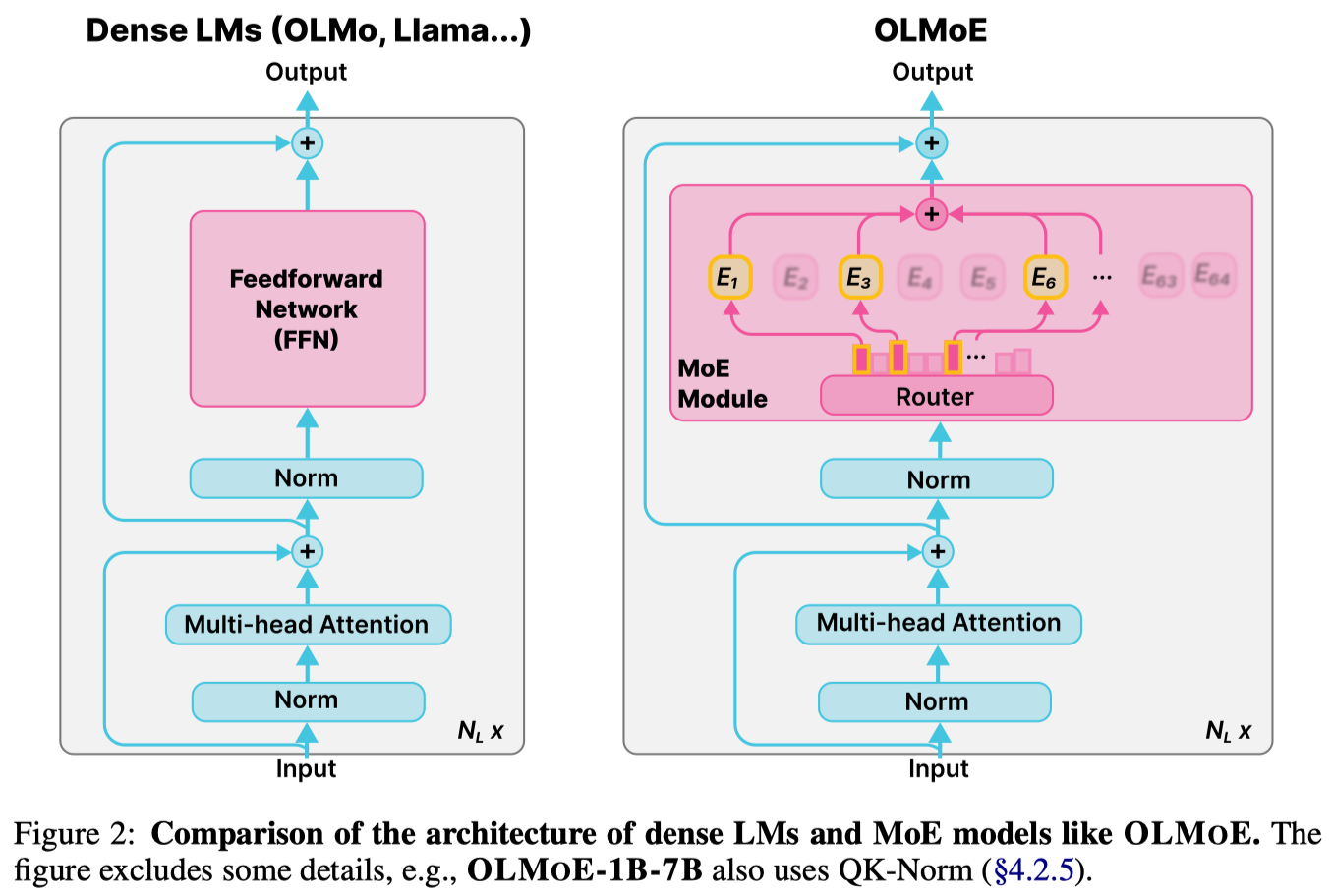
一个 MoE layer 包括两个模块:
- Router:Router 负责为 token 指定合适的专家
- Expert:Expert 负责处理 token
对于输入 $x\in\mathbb{R}^d$, 我们假设有 $N$ 个 Expert,router 一般是一个 linear layer 再加上一个 gating function (softmax 或者 sigmoid, 我们本文中使用 softmax), 其构建了 $\mathbb{R}^d\to\mathbb{R}^N$ 的映射,定义为:
$$ G(x) =[G_1(x),\dots,G_N(x)] = \mathrm{softmax}(W_gx + b)\in\mathbb{R}^N $$其中 $W_g\in\mathbb{R}^{N\times d}$, $b\in\mathbb{R}^N$ 是可学习的参数。$G_{i}(x)$ 代表了当前 token $x$ 选择第 $i$ 个 Expert 的概率。
一般来说,Expert 会使用和 dense 模型一样的 MLP, 我们记为
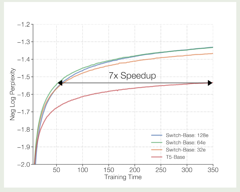
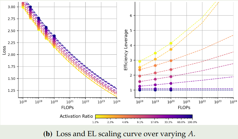
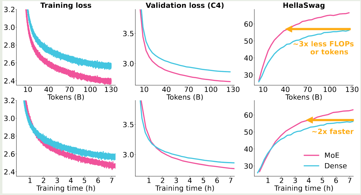
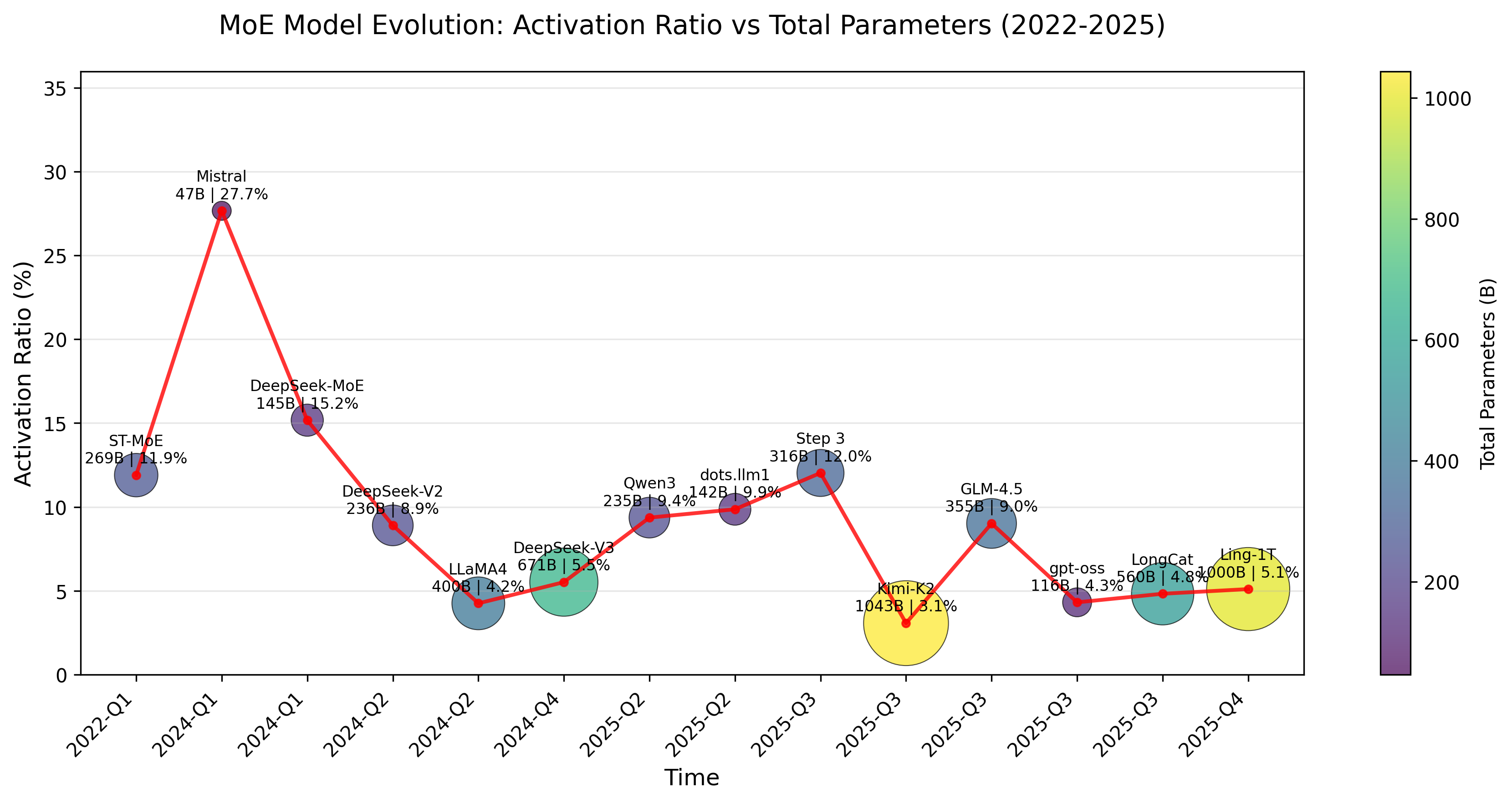
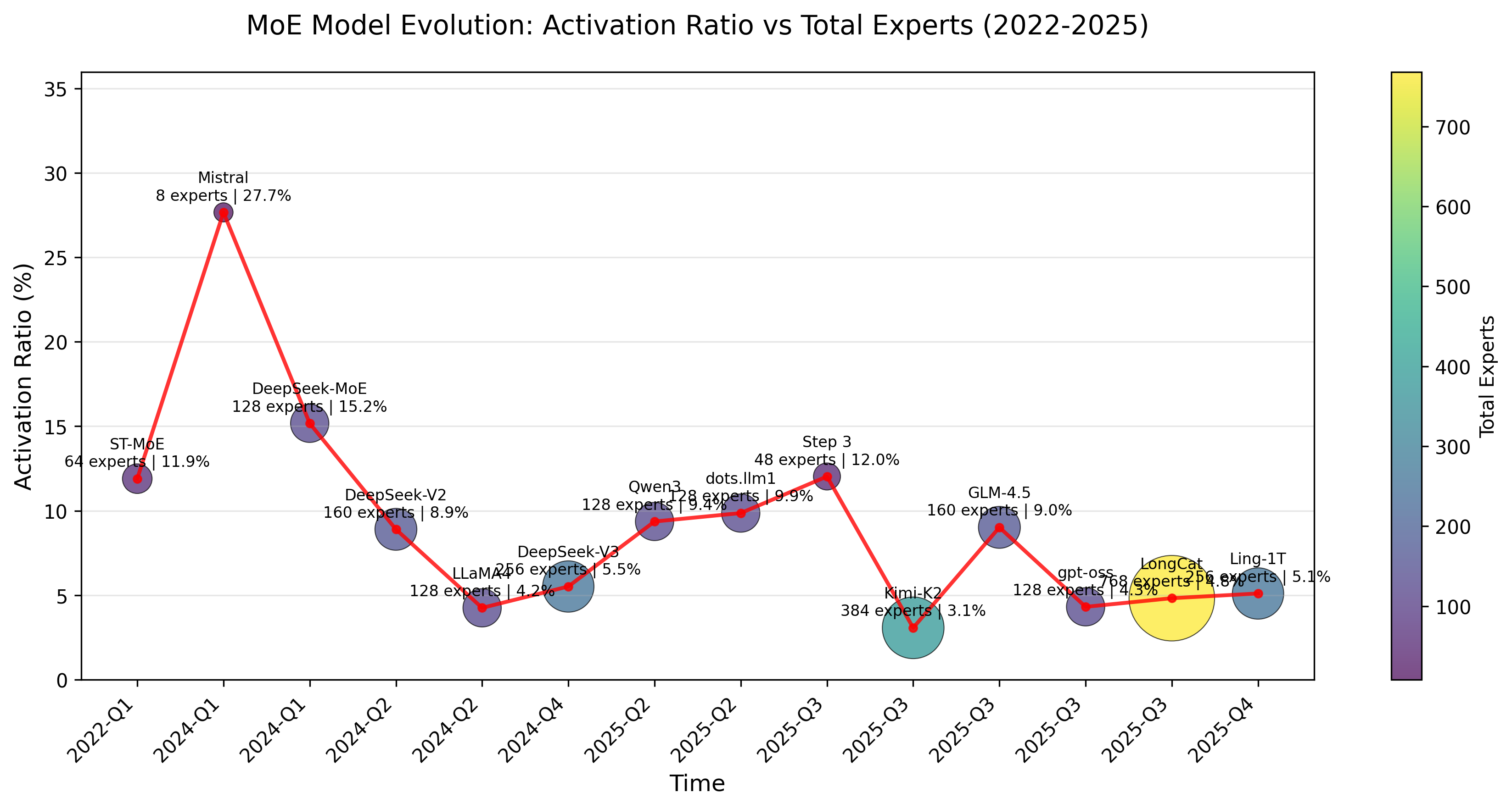
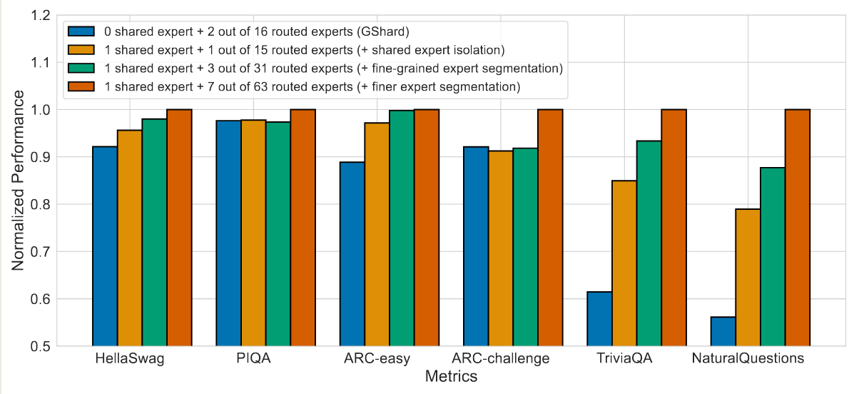
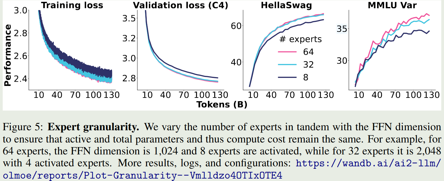
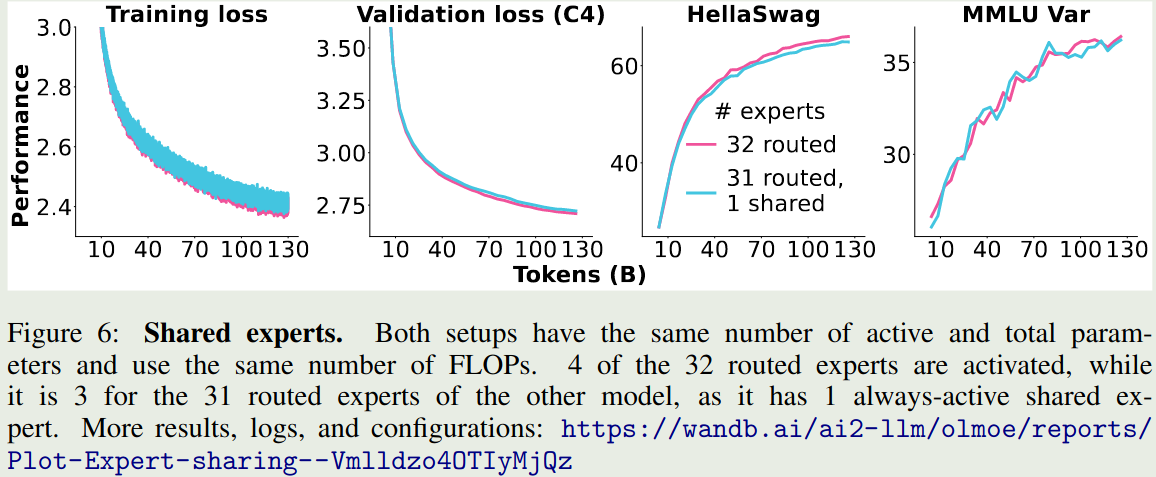
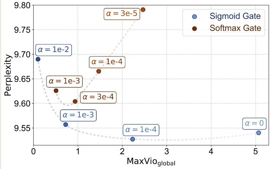
$$ E_i(x) = \mathrm{FFN}(x), \quad i = 1,\dots,N $$接下来,基于 $G(x)$ 和 $E(x)$, 我们会使用合适的方法来挑选 $K 最终 MoE layer 的输出为 这里 $\mathrm{Normalize}(\cdot)$ 代表我们对于输出进行归一化,即 选择 MoE 的原因有三点:效率, scaling law 以及表现。 MoE 训练更加高效,如下图所示 Switch Transformer 的 实验结果说明,MoE model 的训练效率比 dense model 快 7 倍左右。其他模型也有类似结论。总的来说,MoE 模型相比于 dense 模型,训练效率更高。 MoE 模型可以突破传统 scaling law 的限制,在算力固定的情况下,我们可以通过提高 MoE 模型的稀疏度来进一步提高模型的表现 如上图所示,在 FLOPs 给定的情况下,随着模型稀疏度的提高,模型的表现和效率都有提升 MoE 模型的表现更强,如下图所示,MoE 模型的训练,验证损失以及在下游任务上的表现均超过了 dense 模型 激活参数比例变化图如下图所示 可以看到,当前大部分模型的激活比例都在 $5\%$ 左右。 另一方面,从专家的激活比例变化图如下图所示 可以看到,现在大部分模型总专家数都在 200-400 左右,Kimi-k2 认为提高专家个数可以提高模型表现,而 LongCat 则是使用了 phantom expert 机制 一般来说,专家个数越多,模型越稀疏,模型表现越好。扩展专家个数有两个方式: Switch Transformer 也通过实验发现,增加专家个数可以显著提高模型的训练效率和表现,结果如下图所示 可以看到,当我们增加专家个数的时候,模型的表现是持续提升的。并且当我们增加专家个数之后,模型的训练效率也有所提升。 DeepSeekMoE 提出了 fine-granularity expert 的概念,其做法是通过减少 expert 的大小在相同参数量的场景下使用更多的专家。实验结果如下图所示 可以看到,在稀疏度 (激活专家个数占总专家个数比例) 不变的情况下,提高专家的粒度,可以提高模型的表现。 olmoe 对 DeepSeekMoE 的这个观点进行了验证,结果如下图所示, 结果显示,当专家粒度从 8E-1A 扩展到 32E-4A 时,模型在 HellaSwag 上的表现提升了 $10\%$, 但是进一步扩展到 64E-8A 时,模型的表现提升不到 $2\%$, 这说明了无限制提升专家粒度对模型的提升越来越有限。 Kimi-k2 探究了针对 MoE 模型 sparsity 的 scaling law, 结果也说明,提升 sparsity 可以提高模型的表现。因此,其相对于 DeepSeek-V3 使用了 $50\%$ 额外的的专家数。Ling-mini-beta 进一步验证了这个观点。 Shared Expert 由 DeepSeekMoE 提出,其基本思想为,固定某几个专家,响应所有的 token,这样可以让某些专家学习到共有的知识,而让其他的专家学习到特定的知识。这个方法随后被 Qwen1.5, Qwen2 , Qwen2.5 以及 DeepSeek-V3 所采用。 DeepSeekMoE 给出的实验结果如下 作者发现,当使用 shared experts 之后,模型在大部分 benchmark 上的表现都有所提升。 olmoe 在 32 个专家下进行了实验,比较了 4 个激活专家和 3 个激活专家 +1 个共享专家两种设置的表现,结果如下: 作者认为,加入 shared experts 之后,组合的可能性有所减少,这会降低模型的泛化性。因此,在 olmoe 中,作者没有使用 shared experts. 虽然 Qwen1.5, Qwen2 和 Qwen2.5 都使用了 shared experts, 但是后续的 Qwen3 中却并没有使用。 Ling-mini-beta 通过实验得出的结论为,shared expert 应该是一个非零的尽可能小的值,作者认为将 shared expert 设置为 1 是一个比较合理的选择。 一般来说,在选取 top-K 专家时,我们会对 gating layer 的输出进行归一化,通常我们会使用 softmax function: 但是,在 Loss-Free Balancing 中,作者通过实验发现,使用 sigmoid 作为激活函数效果更好,即 其对应的实验结果如下图所示 实验结果显示,sigmoid function 对于超参数更加 robust, 且表现也更好一些。 下面是一些使用不同激活函数的模型例子 Routing Z-loss 由 ST-MoE 提出, Switch Transformer 发现在 gating layer 中使用 其中 $B$ 是 batch size ,$x_j^{(i)}=[W_gx_i+b]_j$ 代表了第 $j$ 个专家对 $i$ 个 token 的激活 logits. olmoe 实验验证结果如下 可以看到,加入 router Z-loss 之后,模型训练的稳定性有所提升,因此 Olmoe 采取了这个改进,但是后续的 MoE 模型使用 Z-loss 较少,个人猜测原因是 Loss-Free Balancing 中提出的加入额外的 loss 会影响 nex-token prediction loss routing 策略直接决定了 MoE 模型的有效性。在为专家分配 token 的时候,我们有如下方式: 三种选择方式如下图所示,图源 MoE survey 每个专家选取 top-k 的 token,此时每个专家处理的 token 个数是相同的,这个方法的好处是自带 load balance。缺点是自回归生成的方式没有完整序列长度的信息,从而导致 token dropping,也就是某些 token 不会被任何专家处理,某些 token 会被多个专家处理。 目前采用这个策略的有 OpenMoE-2, 核心思想是 dLLM 的输出长度固定,expert choice 策略更有效 每个 token 选取 top-k 的专家,好处是每个 token 都会被处理,缺点是容易导致负载不均衡。因此,一般需要加上负载均衡或者 token dropping 策略来提高负载均衡 Capacity Factor
由 Switch Transformer 提出,其定义为 设置 capacity factor 之后,当某个专家处理的 token 个数超过 capacity 之后,概专家的计算就会直接跳过,退化为 residual connection. 后续 DeepSeek-V2 也采用了这种策略,但是 DeepSeek-V3 弃用 Load balancing Loss
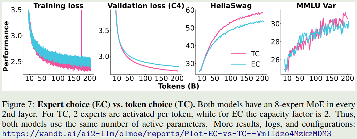
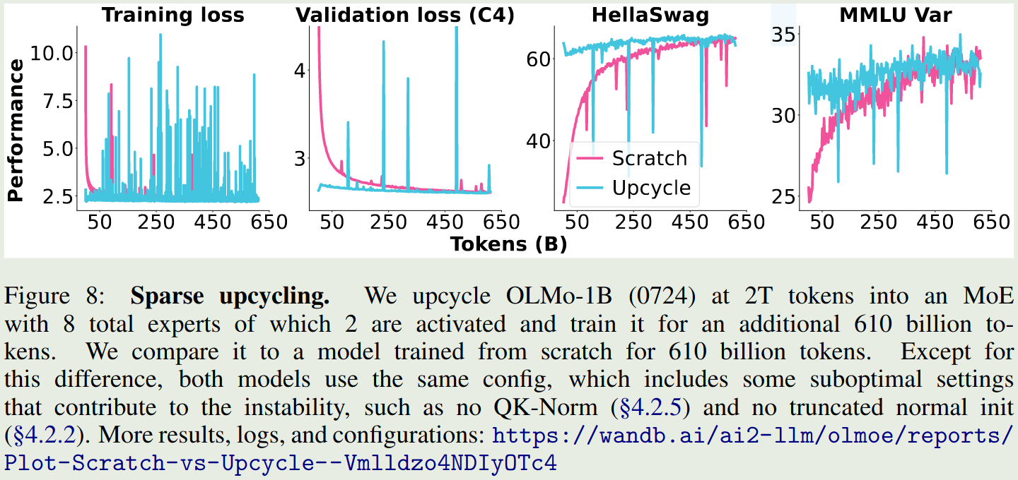
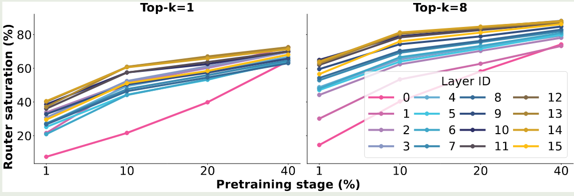
在训练目标中加入负载均衡损失,要求每个专家处理的 token 个数的分布尽可能均匀。 这部分具体见 Load Balancing loss 全局分配决定 token 和专家的匹配关系,后续 Qwen 提出了 Global-batch load balancing 使用了这种方式来提高专家的特化程度 根据输入 token 的难度动态决定激活专家的个数。LongCat 使用了一个 Phantom expert 的方法来实现根据 token 的难度动态分配专家。具体来说,除了 $N$ 个专家之外,MoE 还包括 $Z$ 个 zero-computation expert (现在一共有 $N+Z$ 个专家参与计算), 其计算方式如下 注:LongCat 还是用了 Loss-Free Balancing, 我们这里省略掉了。 现在几乎所有的模型都选择方式 1,即每个 token 选取 top-k 的专家。 olmoe 对比了以下方式 1 和方式 2 的表现,如下图所示 可以看到,加入 load balancing loss 之后,相比于 Expert Choice, Token Choice 的表现更好。但是,expert choice 更加高效,作者认为 expert choice 更适用于多模态,因为丢掉 noise image tokens 对 text token 影响会比较小。因此,在 olmoe 中,作者使用 token choice 作为 routing 策略 upsampling 是一个将 dense model 转化为 MoEmodel 的方法,具体做法就是我们复制 dense model 中的 FFN layer 得到对应 MoE layer 中的 Expert,然后我们再结合 router 训练,这样可以提高整体的训练效率。相关模型有 MiniCPM, Qwen1.5 和 Mixtral MoE (疑似) 实验结果如下图所示 从已有的结果来看,MoE 模型会被 dense 模型的一些超参数所限制,且训练不是很稳定。因此,现在一般不采用这种方法 OpenMoE 分析了 MoE 模型的特化程度,其结论如下 olmoe 探究了训练过程中激活的专家和训练结束后激活的专家的匹配程度,结果如下图所示 实验结果说明,训练 $1\%$ 的数据之后,就有 $40\%$ 的 routing 和训练完毕的 routing 一致,当训练 $40\%$ 的数据之后,这个比例提升到了 $80\%$. 作者认为,这是专家特化的结果,初始的 routing 如果改变的话会带来表现下降,因此模型倾向于使用固定的专家处理特定的 token 作者还发现,later layers 比 early layers 饱和更快,early layer, 特别是 layer 0, 饱和的非常慢。作者认为,这是 DeepSeekMoE 放弃在第一层使用 MoE layer 的原因,因为 load balancing loss 收敛更慢。后续 DeepSeek-V2 和 DeepSeek-V3 均在 early layer 上使用 dense layer 替换掉了 MoE layer MoE 模型的优势在于表现好,但是模型参数往往非常大,为了方便使用,我们需要对训练好的 MoE 模型进行优化,目前主要有蒸馏,专家剪枝/合并以及量化等优化方法 蒸馏是一个将大模型能力传递给小模型的做法,目前已有的包括: 我们这里展示基于 olmoe 的代码,代码如下 针对 MoE 模型的 infra 主要涉及 expert parallelism (EP), EP 将 MoE layer 的计算分为了三个阶段: 其框架图如下所示 在本文中,我们系统性回顾了 MoE 的相关概念,MoE 模型已经是现在大语言模型的主流架构,比如商业模型 Gemini2.5, 开源领先的模型 DeepSeek-V3 , LLaMA4 以及 Qwen3 等都采用了 MoE 的架构,如何进一步优化 MoE 的训练方式是当前研究的一个重点方向。 MoE model information Remark
LongCat 采用了动态激活的方式,因此其结果有一个浮动范围。Why MoE
Efficiency
Scaling Law
Performance
Timeline
MoE Design
Experts Design
Number of Experts
![]()
Shared Experts
Activation Function
Activation function Models softmax Step 3, Kimi-K2, gpt-oss-120B sigmoid GLM-4.5, dots.llm1, DeepSeek-V3 Routing Z-loss
float32 精度可以提高训练稳定性,但是这还不够,因此 ST-MoE 使用了如下的 router Z-loss: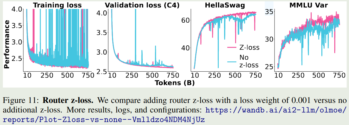
Routing Strategy
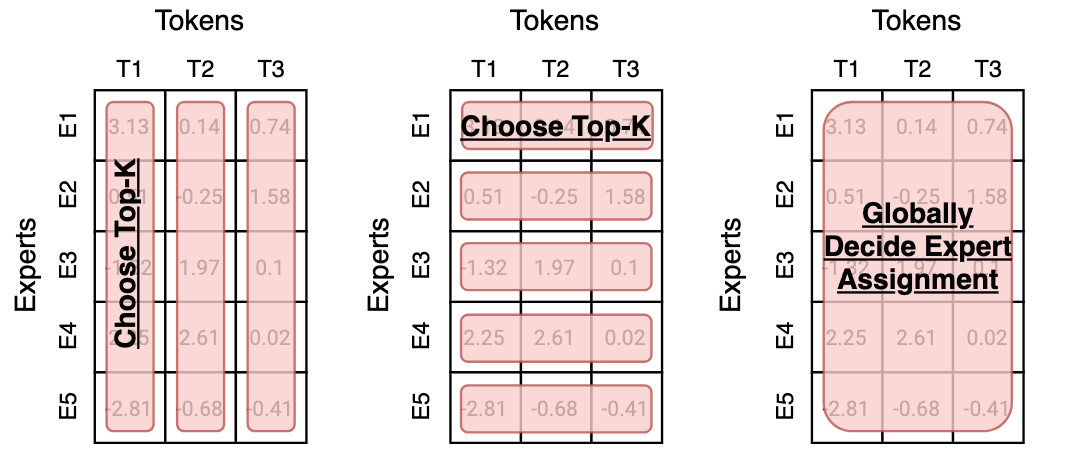
Expert Choice
Token Choice
Global Choice
Dynamic Routing
Overview
Upcycling
Analysis on MoE
Specialization of Experts
Saturation of Experts
Optimization
Code
 1
 2
 3
 4
 5
 6
 7
 8
 9
10
11
12
13
14
15
16
17
18
19
20
21
22
23
24
25
26
27
28
29
30
31
32
33
34
35
36
37
38
39
40
41
42
43
44
45
46
47
48
49
class OlmoeSparseMoeBlock(nn.Module):
    def __init__(self, config):
        super().__init__()
        self.num_experts = config.num_experts
        self.top_k = config.num_experts_per_tok
        self.norm_topk_prob = config.norm_topk_prob
        self.gate = nn.Linear(config.hidden_size, self.num_experts, bias=False)
        self.experts = nn.ModuleList([OlmoeMLP(config) for _ in range(self.num_experts)])

    def forward(self, hidden_states: torch.Tensor) -> torch.Tensor:
        batch_size, sequence_length, hidden_dim = hidden_states.shape
        # hidden_states: (batch * sequence_length, hidden_dim)
        hidden_states = hidden_states.view(-1, hidden_dim)
        # router_logits: (batch * sequence_length, n_experts)
        router_logits = self.gate(hidden_states)

        routing_weights = F.softmax(router_logits, dim=1, dtype=torch.float)
        # routing_weights: (batch * sequence_length, top_k)
        # selected_experts: indices of top_k experts
        routing_weights, selected_experts = torch.topk(routing_weights, self.top_k, dim=-1)
        if self.norm_topk_prob:
            routing_weights /= routing_weights.sum(dim=-1, keepdim=True)
        # we cast back to the input dtype
        routing_weights = routing_weights.to(hidden_states.dtype)

        final_hidden_states = torch.zeros(
            (batch_size * sequence_length, hidden_dim), dtype=hidden_states.dtype, device=hidden_states.device
        )

        # One hot encode the selected experts to create an expert mask
        # this will be used to easily index which expert is going to be selected
        expert_mask = torch.nn.functional.one_hot(selected_experts, num_classes=self.num_experts).permute(2, 1, 0)

        # Loop over all available experts in the model and perform the computation on each expert
        for expert_idx in range(self.num_experts):
            expert_layer = self.experts[expert_idx]
            idx, top_x = torch.where(expert_mask[expert_idx])

            # Index the correct hidden states and compute the expert hidden state for
            # the current expert. We need to make sure to multiply the output hidden
            # states by `routing_weights` on the corresponding tokens (top-1 and top-2)
            current_state = hidden_states[None, top_x].reshape(-1, hidden_dim)
            current_hidden_states = expert_layer(current_state) * routing_weights[top_x, idx, None]

            # However `index_add_` only support torch tensors for indexing so we'll use
            # the `top_x` tensor here.
            final_hidden_states.index_add_(0, top_x, current_hidden_states.to(hidden_states.dtype))
        final_hidden_states = final_hidden_states.reshape(batch_size, sequence_length, hidden_dim)
        return final_hidden_states, router_logits
Infra
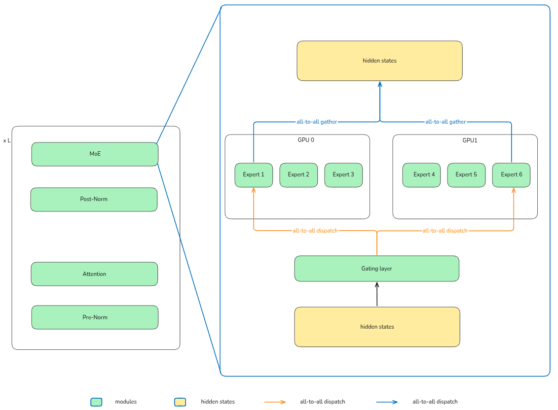
Challenges
Conclusion
Appendix
Model Year total parameters activated parameters shared expert Routed experts activated experts ST-MoE 2022/4 269B 32B 0 64 2 Mistral 2024/1 47B 13B 0 8 2 DeepSeek-MoE 2024/1 145B 22B 4 128 12 DeepSeek-V2 2024/5 236B 21B 2 160 6 LLaMA4 2025/4 400B 17B 1 128 1 DeepSeek-V3 2024/12 671B 37B 1 256 8 Qwen3 2025/5 235B 22B 0 128 8 dots.llm1 2025/6 142B 14B 2 128 6 Step 3 2025/7 316B 38B 1 48 3 Kimi-K2 2025/7 1043B 32B 8 384 1 GLM-4.5 2025/8 355B 32B 1 160 8 gpt-oss 2025/8 116B 5B 0 128 4 LongCat 2025/9 560B 27B* 0 768* 12 Ling-1T 2025/10 1000B 51B 1 256 8 References