Introduction
当我们在硬件上运行算法时,我们的算法效率取决于三个因素:
- 计算机的计算效率,也就是每秒可执行的操作数 (OPs/s)
- 数据移动效率,也就是每秒可传输的 bytes (bytes/s)
- 需要的内存空间 (bytes)
通过分析这三个因素,我们可以给出一个计算的上下界
Arithmetic Intensity
首先,我们要回答的第一个问题是,运行时间意味着什么?为什么实际运行时间比理想时间要更多?
容易知道,实际的运行时间由三部分组成
Computation 首先,运行时间与我们的算法和 GPU 设备相关,在深度学习中,我们的算法通常由 FLOPs 决定,GPU 决定了算法的运行时间:
$$ T_{\mathrm{math}} =\frac{\text{Computation FLOPs}}{\text{Accelerator FLOPs/s}} $$Communication within a chip 其次,运行时间还受加载数据的速度的影响,在执行计算之前,我们需要先把数据从 HBM 加载到对应的 core 上,因此,加载数据的速度也会影响最终运行时间。我们将加载数据的速度称之为 HBM bandwidth.
Communication between chips 最后,当我们在多个 GPU 上运行模型时,我们还需要在 GPU 之间进行通信,相关的通信手段如下表所示 (intra node 代表同一台服务器,inter node 代表不同服务器),我们将 GPU 的通信速度称之为 Network bandwidth.
| Method | Data Path | BandWith | Use cases | |
|---|---|---|---|---|
| Intra Node | NVLink | Direct GPU-to-GPU | 1.8 Tb/s (B200) | TP |
| NVSwith | all-to-all | 900 GB/s-1.8T b/s | full mesh sync in DGX | |
| GPUDirect P2P | Direct over PCIe Bus | 32-128 GB/s | small clusters withou NVLink | |
| Shared Memory | GPU -> CPU RAM -> GPU | 20-50 GB/s | Fallback when P2P is disabled | |
| Inter Node | InfiniBand | GPU -> NIC -> IB Switch | 200-400 Gbps | Large scale LLM training |
| GPU Direct RDMA | GPU -> NIC -> Network | Same as NIC speed | Bypassing CPU for network sync | |
| RoCE (v2) | RAME over Ethernet | 100-400 Gbps | Cost-effective Ethernet clusters | |
| TCP/IP sockets | GPU -> CPU -> Kernel -> Net | < 100 Gbps | Standard networking |
我们将 GPU 的通信 (intra-node 和 inter-node) 效率定义如下
$$ T_{\mathrm{comm}} =\frac{\text{Communication Bytes}}{\text{Network/Memory Bandwith Bytes/s}} $$通常来说,我们可以通过计算 - 通信重叠来降低整体的运行时间,比如说 DeepSeek-V3 等模型提出的优化方法, 此时理论上的最小运行时间就是 $T_{\mathrm{math}}$ 和 $T_{\mathrm{comm}}$ 之间的最大值。另一方面,如果我们不做任何优化,则理论上最大运行时间就是 $T_{\mathrm{math}}$ 和 $T_{\mathrm{comm}}$ 之和。我们定义对应的 bound 如下
$$ \begin{aligned} T_{lower} &= \max(T_{\mathrm{math}} ,T_{\mathrm{comm}} )\\ T_{upper} &= T_{\mathrm{math}}+T_{\mathrm{comm}} \end{aligned} $$注意到
$$ T_{upper} = T_{\mathrm{math}}+T_{\mathrm{comm}} \leq 2\max(T_{\mathrm{math}} ,T_{\mathrm{comm}} )= 2T_{lower} $$也就是最大运行时间最多为最小运行时间的两倍。因此,我们一般直接优化 $T_{lower}$.
如果我们假设我们可以完全达到计算 - 通信重叠,则:
- 当 $T_{\mathrm{math}}>T_{\mathrm{comm}}$ 时, 我们完全利用了 GPU 的资源,因为此时运行时间受硬件的计算效率约束,我们将其称之为 compute bound
- 当 $T_{\mathrm{comm}}> T_{\mathrm{math}}$ 时, 此时运行时间受硬件的通信效率影响,GPU 的(计算)利用率不完全,我们将其称为 communication bound
为了评估一个算法时 compute bound 还是 communication bound, 我们可以使用 arithmetic intensity 来进行评估。我们先分析 single GPU 的情况,再分析 multi GPU 的情况
Single GPU
Arithmetic Intensity 一个算法的 arithmetic intensity 定义为算法通信所需要的 FLOPs 和所需要的 bytes 之比:
$$ \text{Arithmetic Intensity} = \frac{\text{Computation FLOPs}}{\text{Communication Bytes}} $$arithmetic intensity 衡量了一个算法的 FLOPs per bytes, 当 arithmetic intensity 比较高时,说明 $T_{\mathrm{math}}>T_{\mathrm{comm}}$, 此时 GPU 的利用效率较高,反之则说明 GPU 出现了空置的情况。这两种情况的交叉点由 GPU 的 Peak arithmetic intensity 决定:
$$ \begin{aligned} T_{\mathrm{math}}=T_{\mathrm{comm}} &\Leftrightarrow \frac{\text{Computation FLOPs}}{\text{Accelerator FLOPs/s}} = \frac{\text{Communication Bytes}}{\text{Bandwith Bytes/s}}\\ &\Leftrightarrow \frac{\text{Computation FLOPs}}{\text{Communication Bytes}} = \frac{\text{Accelerator FLOPs/s}}{\text{Bandwith Bytes/s}}\\ &\Leftrightarrow \text{Intensity}(\text{Computation}) = \text{Intensity}(\text{GPU}) \end{aligned} $$这里 $\text{Intensity}(\text{GPU})$ 就是 GPU 达到 peak FLOPs 时对应的 arithmetic intensity.
不同 GPU Tensor Core 对应的 intensity 如下所示
| GPU | Generation | bandwidth | peak BF16 Tensor Core | intensity |
|---|---|---|---|---|
| V100 | Volta | 300 GB/s | 125 TFLOPs/s | 427 |
| A100 | Amper | 1,935 GB/s | 156 TFLOPs/s | 83 |
| H100 | Hopper | 3.35TB/s | 495 TFLOPs/s | 147 |
| H200 | Hopper | 4.8TB/s | 495 TFLOPs/s | 147 |
| B200 | Blackwell | 576 TB/s | 2250 TFLOPs/s | 3.9 |
Example 假设我们使用 BF16 精度计算两个长度为 $N$ 的向量的内积,计算时的流程如下:
- 从 HBM 中加载两个向量,通信量为 $2*2N$
- 计算两个向量内积,需要 $N$ 次乘法和 $N-1$ 次加法
- 将结果写回 HBM, 通信量为 $2$.
从而内积的 intensity 为
$$ \text{Intensity}(\text{dot product}) = \frac{\text{Total FLOPs}}{\text{Total Bytes}} = \frac{N+N-1}{2N+2N+2} = \frac{2N-1}{4N+2}\to \frac12 $$也就是说,内积的 arithmetic intensity 最大为 $1/2$, 说明这是一个 memory-bound operation.
接下来,我们可以对 communication-bound 和 compute-bound 进行可视化,如下图所示
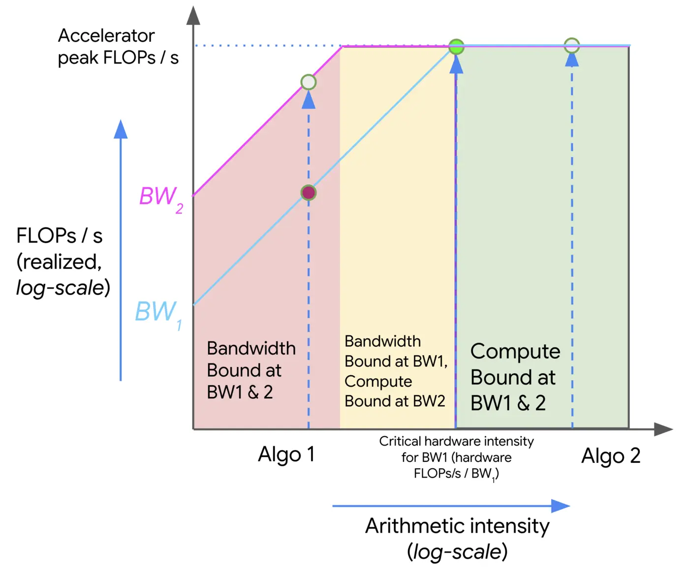
这里我们展示了两个算法 Algo 1 和 Algo 2 的 arithmetic intensity, 当 intensity 较小(小于硬件的 intensity)是,算法为 communication bound, 随着 intensity 增加,算法逐渐由 communication bound 过渡到 compute bound. 上面这个模型被称为 Roofline model, 其展示了算法计算效率与硬件之间的关系。
为了提高算法计算效率,我们可以通过提升算法的 arithmetic intensity 或者提高 memory bandwith.
Example
接下来我们来看一下矩阵计算的 intensity, 我们仍然假设在 BF16 精度下进行计算,假设输入矩阵为 $X\in\mathbb{R}^{b\times d}$ 以及 $Y\in\mathbb{R}^{d\times f}$ , 则输出为 $Z=XY\in\mathbb{R}^{b\times f}$. 计算过程为:
- 从 HBM 中加载 $X$ 和 $Y$, 通信量为 $2df+2bd$ bytes
- 计算矩阵乘法,计算量为 $2bdf$ FLOPs
- 将结果写回到 HBM, 通信量为 $2bf$.
因此对应的 intensity 为
$$ \text{Intensity}(\text{MatMul}) = \frac{2bdf}{2bd+2df+2bf} = \frac{bfd}{bd+df+bf} $$假设 $b << \min(d,f)$ (在 LLM 中这个假设一般成立),我们有
$$ \text{Intensity}(\text{MatMul}) = \frac{bfd}{bd+df+bf}\approx \frac{bdf}{df}=b $$因此我们就可以通过调整 $b$ (batch size) 来将算法从 memory-bound 转换为 compute bound.
Multi GPU
在 multi GPU 的场景下,我们需要关注 GPU 之间通信的效率,一般来说,GPU 之间效率要远小于 GPU 内部通信效率,下面是不同 GPU 的内部通信(HBM bandwidth) 和 GPU 之间通信效率对比
| GPU | Generation | HBM Type | HBM bandwidth | NVLink Generation | NVLink Bandwidth |
|---|---|---|---|---|---|
| V100 | Volta | HBM2 | 300 GB/s | 2.0 | 300 GB/s |
| A100 | Amper | HBM2e | 1,935 GB/s | 3.0 | 600 GB/s |
| H100 | Hopper | HBM3 | 3.35TB/s | 4.0 | 900 GB/s |
| H200 | Hopper | HBM3e | 4.8TB/s | 4.0 | 900 GB/s |
| B200 | Blackwell | HBM3e | 576 TB/s | 5.0 | 1800 GB/s |
Example 我们考虑一个分布式矩阵乘法,假设我们有两个 GPU, 计算精度为 BF16, 矩阵 $X\in\mathbb{R}^{b\times d}$ 以及 $Y\in\mathbb{R}^{d\times f}$ 分别被切分为相同大小存储在这两个 GPU 上,此时,计算流程为:
- 在 GPU0/GPU1 上,分别从对应的 HBM 中加载 $X_1, Y_1$ 以及 $X_2, Y_2$
- 在 GPU0/GPU1 上,分别计算对应的矩阵乘法 $A=X_1Y_1\in\mathbb{R}^{b\times f}$ 和 $B=X_2Y_2\in\mathbb{R}^{b\times f}$, 计算量为 $2bdf$.
- 将 GPU1 的结果 $B$ 通信传输到 GPU0 上,通信量为 $2bf$.
- 对结果进行相加,$Z=A+B$. 计算量为 $bf$.
此时,我们的 intensity 为 (注意这里计算时间除以 2 代表我们使用两张 GPU 因而效率翻倍了)
$$ \text{Intensity}(\text{MatMul (2-GPU)}) = \frac{2bfd/2}{2bf}= \frac{d}{2} $$可以看到,此时决定性因素在于 $d$ 而不是 $b$, 这对于我们实现并行算法至关重要