Introduction

softmax 函数用于将 $K$ 个实数转换为一个 $K$ 维概率分布。其具体做法是先对所有元素指数化，即求 $e^x$, 然后每个元素除以所有指数的和。即

Analysis

Properties

softmax 的第一个性质是 shift invariance, 即

证明比较容易：

Gradient

向量输入下 Softmax 函数的 Jacobian 矩阵推导

设输入为向量 $\mathbf{z} = [z_1, z_2, \dots, z_d]^\top \in \mathbb{R}^d$，Softmax 函数的输出为向量 $\mathbf{a} = [a_1, a_2, \dots, a_d]^\top \in \mathbb{R}^d$，其中每个元素定义为：

记分母（归一化因子）为 $S = \sum_{k=1}^d e^{z_k}$，则 $a_j = e^{z_j}/S$.

我们分两种情况计算 $\frac{\partial a_j}{\partial z_k}$：

当 $j = k$ 时， 此时求 $a_j$ 对自身输入 $z_j$ 的偏导数：

当 $j \neq k$ 时， 此时求 $a_j$ 对输入 $z_k$ 的偏导数有：

综合以上两种情况，Jacobian 矩阵 $\mathbf{J}$ 可表示为：

Interpretation

Soft Argmax

softmax 是 argmax 的 smooth approximation, 所以实际上 softmax 指的是 “soft argmax". 为了证明这一点，我们首先定义如下函数

易知， $\mathrm{softmax}(\mathbf{z})=\mathrm{softmax}(\mathbf{z};1)$. 并且，$\mathrm{softmax}$ 还是一个光滑函数

我们定义 smooth approximation 为

Definition 如果 $\lim_{\tau\to0^+}\mathrm{softmax}(\mathbf{z};\tau)=\mathbb{1}{\arg\max(\mathbf{z})}$, 则我们说 $\mathrm{softmax}(\cdot;\tau)$ 是 $\arg\max$ 的光滑近似，特别地，$\mathrm{softmax}(\cdot)$ 是 $\arg\max$ 的光滑近似。这里 $\arg\max(\mathbf{z})=\arg\max_k z_k$ 是最大值的索引，$\mathbb{1}\in{0,1}^K$ 是示性函数 (indicator function), 即 $\mathbb{1}{\arg\max(\mathbf{z})}[i]=1$ 当且仅当 $z_i=\max_jz_j$.

我们下面来进行证明。我们不妨假设最大值唯一，其 index 为 $m$, 即 $z_m = \max_i z_i$. 由前面的性质，我们有：

此时，我们有

当最大值不唯一的时候，我们记 $\mathcal{I} = {i\in[K]\mid z_i=\max_j z_j}$, 与上面方法类似，最终 $\mathrm{softmax}(\cdot;\tau)$ 的结果为

因此，我们就证明了 softmax 是 argmax 函数的 smooth approximation.

Statistical Mechanics

Temperature

我们前面介绍了 $\mathrm{softmax}(\mathbf{z};\tau)$ 函数，这里的 $\tau$ 实际上被称为温度 (temperature), 它控制了输入的 variance, $T$ 越大，输入的 variance 越低，输出就倾向于均匀分布，而 $T$ 越小，则说明输入的 variance 越高，输出就倾向于 one-hot 分布。

我们前面已经证明了后者，现在我们来证明一下前者，证明思路也很简单，$T\to+\infty$ 时，$e^{x/T}\to 1$, 因而

下面是可视化的代码以及结果

 1
 2
 3
 4
 5
 6
 7
 8
 9
10
11
12
13
14
15
16
17
18
19
20
21
22
23
24
25
26
27
28
29
30
31
32
33
34
35
36

import numpy as np
import matplotlib.pyplot as plt
from scipy.interpolate import make_interp_spline

def softmax(x):
    e_x = np.exp(x - np.max(x))
    return e_x / e_x.sum()

num_elements = 15
indices = np.arange(num_elements)
logits = np.linspace(-3.5, 3.5, num_elements)
scales = [0.01, 0.1, 1.0, 5.0, 10.0, 100.0]

plt.figure(figsize=(10, 6))

for s in scales:
    probs = softmax(logits * s)
    
    x_smooth = np.linspace(indices.min(), indices.max(), 300)
    spl = make_interp_spline(indices, probs, k=3)
    y_smooth = np.clip(spl(x_smooth), 0, None) # Clip to ensure no negative artifacts
    
    plt.plot(x_smooth, y_smooth, label=f'Scale = {s}', linewidth=2)

uniform_prob = 1.0 / len(indices)
plt.axhline(y=uniform_prob, color='black', linestyle=':', alpha=0.6, label=f'Uniform distribution')

plt.xticks(indices)
plt.xlabel('Logit Index', fontsize=12)
plt.ylabel('Softmax Probability', fontsize=12)
plt.title('Impact of Variance Scaling on Softmax Distribution', fontsize=14)
plt.legend(title="Variance Scale")
plt.grid(True, linestyle='--', alpha=0.5)
plt.tight_layout()

plt.show()

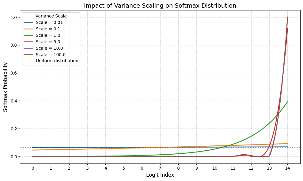
可以看到，当 variance 比较小的时候，输出的分布接近于均匀分布，而 variance 越大，输出的分布越接近 One-hot 分布。

在 attention 的计算过程中，我们也有 softmax 函数，为了在 softmax 过程中避免 variance 的影响，现在会在计算 softmax 之前加入 normalization layer 来提前进行归一化。见 QK-norm.

Algorithms

Implementation

由于 $e^x$ 在实际计算时，非常容易溢出，因此在实现的时候，我们往往会考虑其数值稳定性。实际上，现在的 softmax 函数基本由 logsumexp 实现，logsumexp 函数定义如下

softmax 函数与 logsumexp 函数的关系如下

考虑前面提到的 $e^x$ 数值溢出的问题，我们的输入会先经过 shift, 减掉最大值。此时我们有

这里我们使用了前面推导出来的 shift invariance 性质。对应的代码实现如下：

1
2
3
4

def softmax(x: torch.Tensor, dim: int = -1) -> torch.Tensor:
    x = x - x.max(dim=dim, keepdim=True).values
    log_sum_exp = torch.log(torch.sum(torch.exp(x), dim=dim, keepdim=True))
    return torch.exp(x - log_sum_exp)

Gumbel-softmax Reparametrization Trick

见 Reparameterization

Online Softmax

注意到我们在计算 softmax 时，需要加载 $\mathbf{z}$ 的全部信息，如果 $\mathbf{z}$ 非常大的话，会产生频繁的内存读写进而影响整体效率。因此 flash attention 中提出了 online softmax 算法来减少内存访问开销。

其具体做法是假设我们的输入被分为若干个 block, 即 $\mathbf{z}=[\mathbf{z}^1;\dots,\mathbf{z}^n]\in\mathbb{R}^K$, 这里 $\mathbf{z}^i\in\mathbb{R}^{K/n}$ ($K\mod n=0$).

对于 $\mathbf{z}\in\mathbb{R}^K$, flash attention 定义如下结果

对于 $\mathbf{z}=[\mathbf{z}^1;\dots,\mathbf{z}^n]\in\mathbb{R}^K$, 我们现在的计算方式为

因此，如果我们额外记录 $m(x)$ 以及 $\ell(x)$ 这两个量，那么我们可以每次仅计算 softmax 的一个 block. 计算完毕之后，$m_i(\mathbf{z})$ 和 $\ell_i(\mathbf{z})$ 就分别代表了 global max 和 global denominator.

Conclusion

我们回顾了机器学习中 softmax function 的基本定义与性质

References

• Softmax function
• Softmax to the Max
• Online normalizer calculation for softmax